Electrical Engineering BMT & UFC › Charging a Storage Element

Capacitor and Resistor

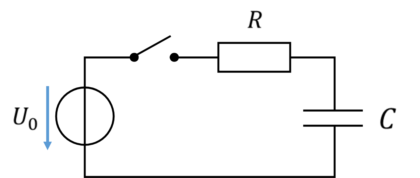
For simplicity, we consider the case in which there is only a resistor between an ideal voltage source and a capacitor. Let us look at the mesh equation and the component equations of the circuit. The following applies

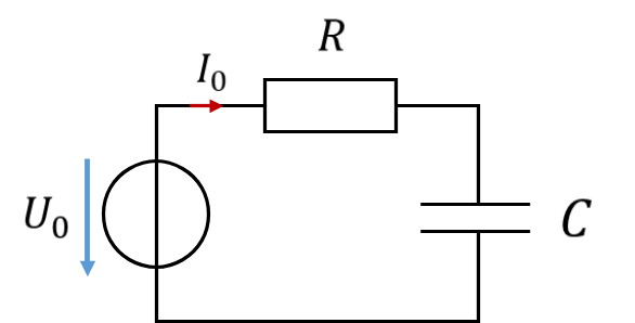
Series connection of voltage source U0, resistor R and capacitor C

\[ \begin{gathered} U_0 = U_R + U_C \\[4pt] I_0 = I_R = I_C \\[4pt] U_R = R \cdot I_0 \\[4pt] U_C = U_0 - U_R = U_0 - R \cdot I_0 \end{gathered} \]

Let us first look at the empty capacitor with U_C = 0 V. The voltage across the resistor then equals the voltage of the source. There is no operating point at which more voltage drops across the resistor. That is why the current is at its maximum when the capacitor is empty.

\[ \begin{gathered} \text{Empty capacitor: } U_C = 0\,\mathrm{V} \\[4pt] U_R = U_0 - U_C = U_0 \\[4pt] I_0 = \frac{U_0}{R} \text{ maximum} \end{gathered} \]

The current charges the capacitor. Current flows into the capacitor until it is charged to the source voltage. No more voltage can be present across the capacitor. Next, let us look at a fully charged capacitor:

\[ \begin{gathered} \text{Fully charged capacitor: } U_C = U_0 \\[4pt] U_R = U_0 - U_C = 0\,\mathrm{V} \\[4pt] I_0 = \frac{U_R}{R} = 0\,\mathrm{A} \end{gathered} \]

At this operating point, no current flows. The potentials to the left and right of the resistor are equal. No voltage drops across the resistor any more, so the current through the resistor is 0. The voltage across the resistor depends on how much voltage drops across the capacitor, i.e. how far it is already charged. The higher the capacitor voltage, the smaller the current becomes.

With this insight, we switch to the water model for an intuitive explanation.

Water model

Note: this section up to the next heading is not relevant for the exam, but it helps a lot with understanding.

We consider a very large, shallow lake at a fixed height, which represents an ideal voltage source for water. This lake keeps its height and its fill level regardless of how much water is taken from it. A water store (bucket) is filled from this lake via a pipe. This corresponds to the electrical circuit diagram.

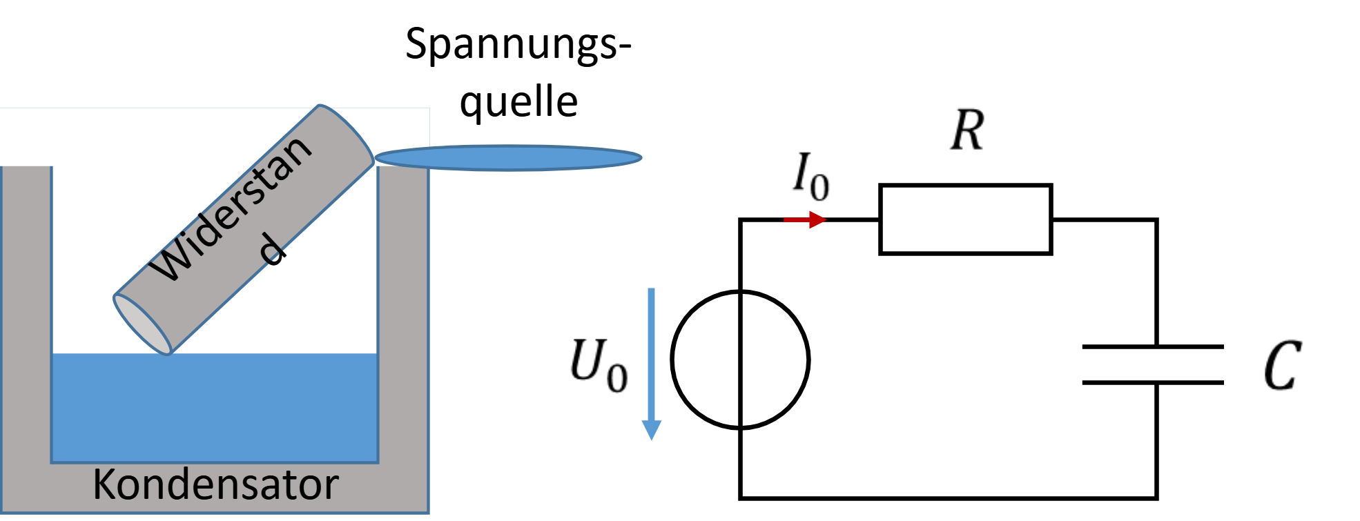
Water model: capacitor as a basin, resistor as a pipe, voltage source as a water level — Spannungsquelle = voltage source · Kondensator = capacitor

The voltage of the source corresponds to the height of the lake. It does not change. The voltage of the capacitor corresponds to the fill height of the store. The voltage across the resistor corresponds to the slope of the pipe, i.e. the difference in height between the pipe ends.

In the series connection of R and C, the source voltage is divided between the resistor and the capacitor. In the analogy, the height of the lake must therefore be divided between the fill height of the store and the slope of the pipe. That is why the lower end of the pipe floats on the water in the store. The slope of the pipe thus becomes smaller the higher the store is filled.

If the store is empty, the slope of the pipe is at its maximum. So the maximum amount of water flows into the store. If the store is full, there is no slope left for the pipe. No more water flows into the store. The fuller the store, the lower the inflow through the pipe, because its slope decreases. This is how charging a capacitor via a resistor works, illustrated intuitively.

The following figure shows numerical values for the electrical quantities and graphics for the respective fill levels of the capacitor in the water model:

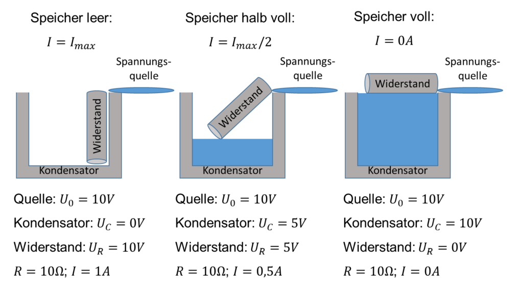
Store empty, half full and full: voltages and currents in the water model — Speicher = storage element · Quelle = source · Kondensator = capacitor · Widerstand = resistor · Spannungsquelle = voltage source

In the left picture, the bucket is empty. The pipe has its maximum slope, and the maximum amount of water flows into the bucket. This corresponds to a resistor whose voltage is at its maximum when the capacitor is empty and through which the maximum current therefore flows into the capacitor.

The fuller the bucket becomes, the smaller the slope of the pipe, so less and less water flows into the bucket (middle picture). When the fill level of the bucket reaches the height of the source, the slope of the pipe is 0, so no more water flows into the bucket. This is shown in the right picture.

Time curves

The time curve of a filling process looks roughly like this:

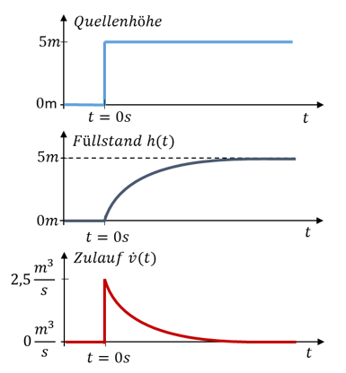
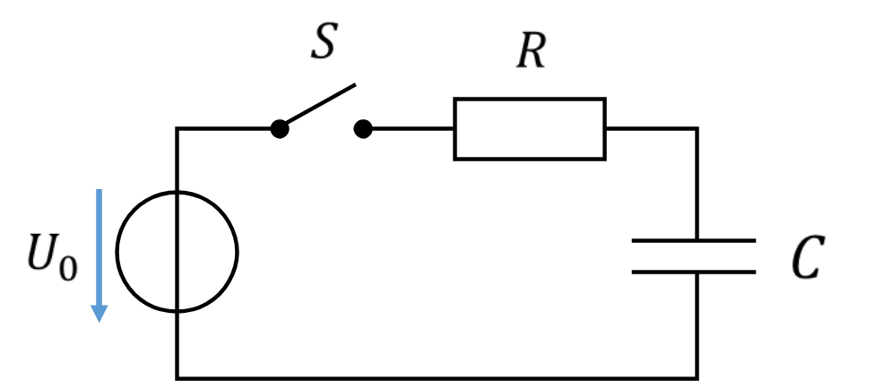
Source height, fill level h(t) and inflow v̇(t) over time — Quellenhöhe = source height · Füllstand = level · Zulauf = inflow

\[ \begin{gathered} \text{Example: } h_{\mathrm{Max}} = 5\,\mathrm{m} \\[4pt] \text{Pipe with } R = 2\,\frac{\mathrm{s}}{\mathrm{m}^2} \text{ “resistance”} \\[4pt] \text{Maximum inflow: } \dot{v}_{\mathrm{Max}} = \frac{h_{\mathrm{Max}}}{R} = \frac{5\,\mathrm{m}}{2\,\dfrac{\mathrm{s}}{\mathrm{m}^2}} = 2.5\,\frac{\mathrm{m}^3}{\mathrm{s}} \end{gathered} \]

To calculate the charging process, we need a switch. If the store were permanently connected to the source, it would simply always be charged. That is boring. Instead, the source is connected to the empty store by closing a switch (for water: a valve) at the time t = 1 s. In electrical engineering, a voltage source is connected via a switch to the series connection of resistor and capacitor.

Mathematical treatment

The mathematical treatment in this section up to the next heading is not relevant for the exam. The solution of the problem is described by a differential equation. You probably lack the mathematical basis for this. So simply try to follow the calculation more or less.

From now on, I use lower-case letters for voltage and current in the calculations. We use upper-case letters for constant values that do not change over time. When the capacitor is charged and discharged, voltage and current change over time, which is why I use lower-case letters. Only the constant source voltage and the constant initial voltage of the capacitor can still be written in upper case.

In the series connection of resistor and capacitor, the following equations apply:

\[ \begin{gathered} U_0 = u_R(t) + u_C(t) \\[4pt] i_0(t) = i_R(t) = i_C(t) \\[4pt] u_R(t) = R \cdot i_0(t) \\[4pt] u_C(t) = \frac{1}{C} \int i_0(t)\,dt + U_{C0} \\[6pt] U_0 = u_R(t) + u_C(t) = R \cdot i_0(t) + \frac{1}{C} \int i_0(t)\,dt + U_{C0} \end{gathered} \]

In the bottom equation, the current and its integral appear in one equation. Differentiating it once gives an equation containing the current and its derivative. This type of equation is called a differential equation. I will not derive the solution; I simply state the result. Then we check the result for plausibility by substituting it into the equation. For the current, the following applies:

\[ \begin{gathered} i_0(t) = \frac{U_0}{R} \cdot e^{-\frac{t}{\tau}} \text{ with } \tau = R \cdot C \\[6pt] \text{Substituting into the formula with } U_{C0} = 0\,\mathrm{V}\text{:} \\[4pt] U_0 = u_R(t) + u_C(t) \\[4pt] U_0 = R \cdot i_0(t) + \frac{1}{C} \int i_0(t)\,dt + U_{C0} \\[4pt] U_0 = R \cdot \frac{U_0}{R} \cdot e^{-\frac{t}{\tau}} + \frac{1}{C} \int \left(\frac{U_0}{R} \cdot e^{-\frac{t}{\tau}}\right) dt \\[6pt] \frac{U_0}{R} \text{ is constant and is taken out in front of the integral:} \\[4pt] U_0 = U_0 \cdot e^{-\frac{t}{\tau}} + \frac{U_0}{RC} \int \left(e^{-\frac{t}{\tau}}\right) dt \\[6pt] \text{Solving the antiderivative with } \int \left(e^{-kt}\right) dt = \frac{1}{-k} e^{-kt} + c \\[4pt] \text{with } k = \frac{1}{\tau} = \frac{1}{RC} \text{ and } c = \tau \text{ (from } u_C(0) = 0\,\mathrm{V}\text{)} \\[6pt] U_0 = U_0 \cdot e^{-\frac{t}{\tau}} + \frac{U_0}{RC} \cdot \left[(-\tau) \cdot e^{-\frac{t}{\tau}} + \tau\right] = \left(U_0 - \frac{U_0}{RC} \cdot RC\right) \cdot e^{-\frac{t}{\tau}} + U_0 \\[6pt] U_0 = (U_0 - U_0) \cdot e^{-\frac{t}{\tau}} + U_0 = U_0 \end{gathered} \]

Because the equation is satisfied in the last line with U₀ = U₀, we have evidently substituted something correct for i₀. Otherwise the left and right sides of the equation would not be equal after substitution. This shows that the upper equation for the current is correct. For the voltage across the empty capacitor with U_C0 = 0 V, the following then applies:

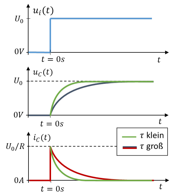
\[ \begin{aligned} u_C(t) &= \frac{1}{C} \int i_0(t)\,dt = \frac{1}{C} \int \left(\frac{U_0}{R} \cdot e^{-\frac{t}{\tau}}\right) dt \\[4pt] &= \frac{U_0}{RC} \cdot (-\tau) \cdot e^{-\frac{t}{\tau}} + \frac{U_0}{RC} \cdot RC \\[4pt] &= -U_0 \cdot e^{-\frac{t}{\tau}} + U_0 \\[4pt] &= U_0 \left(1 - e^{-t/\tau}\right) \end{aligned} \]

The curves of voltage and current at the capacitor correspond to those at the store in the water model. To be able to model connecting the source via switch S better, I introduce an internal voltage u_i. With the switch open, u_i = 0 V. With the switch closed, u_i = U₀. The switch is closed at t = 0 s.

RC circuit with input voltage ui and capacitor voltage uC

\[ \begin{gathered} u_C(t) = U_0 \left(1 - e^{-t/\tau}\right) \\[4pt] i_0(t) = \frac{U_0}{R} \cdot e^{-\frac{t}{\tau}} \\[4pt] \tau = R \cdot C \end{gathered} \]

Simulation

Time curves of ui(t), uC(t) and i0(t) during charging

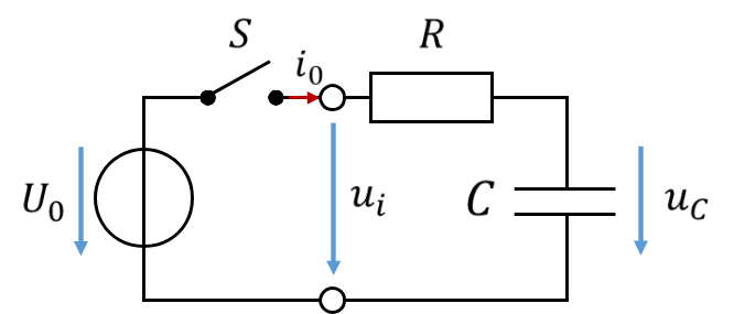
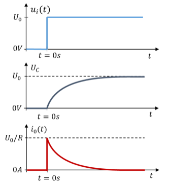
Let us look at the electrical quantities at the switching instant and after an infinitely long time. To do this, we substitute the values 0 s and ∞ for the time t. The following applies:

\[ \begin{gathered} e^{0} = 1 \\ e^{-\infty} = 0 \\ u_C(t) = U_0 \left(1 - e^{-t/\tau}\right) \\ i_0(t) = \frac{U_0}{R} \cdot e^{-\frac{t}{\tau}} \\[4pt] \text{After an infinitely long time for } t \rightarrow \infty\text{:} \\ i_C(\infty) = \frac{U_0}{R} \cdot 0 = 0\,\mathrm{A} \\ u_C(\infty) = U_0 (1 - 0) = U_0 \end{gathered} \]

\[ \begin{gathered} \text{At the switching instant at } t = 0\,\mathrm{s}\text{:} \\ i_C(0\,\mathrm{s}) = \frac{U_0}{R} \cdot 1 = \frac{U_0}{R} \\ u_C(0\,\mathrm{s}) = U_0 (1 - 1) = 0\,\mathrm{V} \end{gathered} \]

Discharging a capacitor

So far, we have only charged the capacitor. A capacitor is usually discharged into a load. This load often behaves like an ohmic resistor. That is why only the case of a capacitor discharging via a resistor is investigated here. Again, simplifying assumptions are made:

At the start of the discharge process, the capacitor is charged to a voltage U_C = U₀. It is initially decoupled from the load by a switch and therefore maintains its voltage.

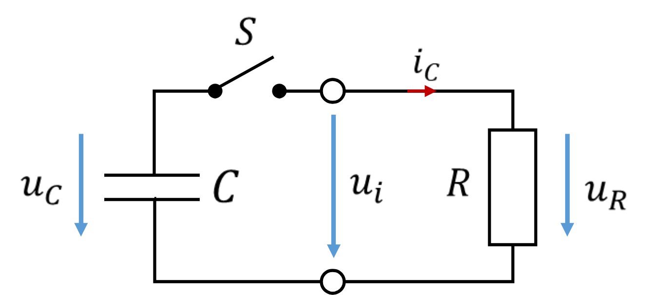
Discharging: capacitor C via switch S and resistor R

Now we close the switch and look at the voltage and current while the capacitor discharges. I have again drawn the auxiliary quantity u_i behind the switch.

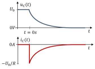
With the switch open, u_i = 0 V. With switch S closed, the capacitor and the resistor are connected in parallel. Then u_i = u_R. The equations for current and voltage during discharging are (again without derivation):

\[ \begin{gathered} u_C(t) = U_0 \cdot e^{-t/\tau} \\[4pt] i_0(t) = -\frac{U_0}{R} \cdot e^{-\frac{t}{\tau}} \\[4pt] \tau = R \cdot C \end{gathered} \]

Let us again look at the simple points in time t = 0 s and t → ∞ to check the equations for plausibility. As soon as switch S is closed, the capacitor voltage is applied to the resistor. The voltage across the resistor is never greater than now. That is why the maximum current flows out of the capacitor. After an infinitely long time, the capacitor is completely discharged. Then there is no more voltage across the resistor either. So the current is then 0 A.

\[ \begin{gathered} e^{0} = 1 \\ e^{-\infty} = 0 \\ u_C(t) = U_0 \cdot e^{-t/\tau} \\ i_C(t) = -\frac{U_0}{R} \cdot e^{-\frac{t}{\tau}} \\[4pt] \text{After an infinitely long time for } t \rightarrow \infty\text{:} \\ i_C(\infty) = -\frac{U_0}{R} \cdot 0 = 0\,\mathrm{A} \\ u_C(\infty) = U_0 \cdot 0 = 0\,\mathrm{V} \end{gathered} \]

\[ \begin{gathered} \text{At the switching instant at } t = 0\,\mathrm{s}\text{:} \\ i_C(0\,\mathrm{s}) = -\frac{U_0}{R} \cdot 1 = -\frac{U_0}{R} \\ u_C(0\,\mathrm{s}) = U_0 \cdot 1 = U_0 \end{gathered} \]

Time curves of uC(t) and iC(t) during discharging

The meaning of tau (τ)

Note: from here on, the text is relevant for the exam again.
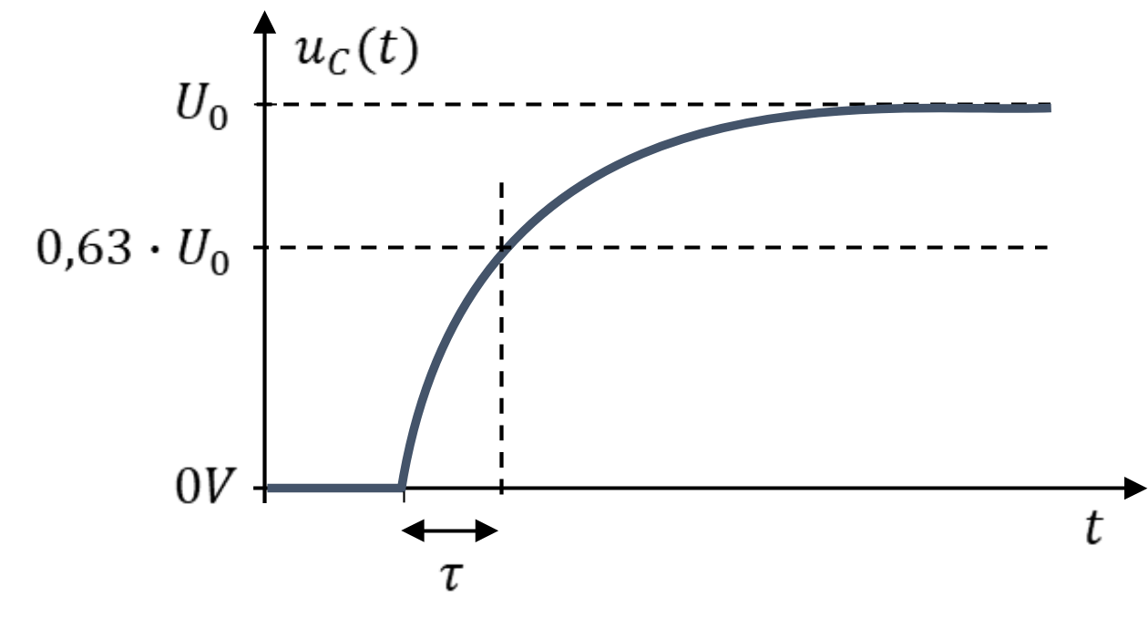
Tau has the unit second, so it is a time quantity. It describes how slowly or quickly a charging process takes place. The larger tau is, the more time passes until the capacitor is fully charged, i.e. the slower the process. The shape of the charging curve does not change with tau.

The following applies: τ = RC. The larger the capacitance C of the capacitor, the slower the charging process. According to Q = C ∙ U, more charges have to be separated until the capacitor reaches its target voltage. A larger resistance reduces the charging current, which is why charging takes longer.

Influence of the time constant τ on uC(t) and iC(t) — klein = small · groß = large

At the time t = τ, the capacitor voltage reaches 63 % of its final value. So during charging, u_C(τ) = 0.63 ∙ U₀ at t = τ. The value of τ can be read off the time curve. It is the time difference between the moment the switch is flipped and the moment the capacitor voltage has reached 63 % of its final value.

Time constant τ: after t = τ, the capacitor is charged to 63 % of U0

Let us look at the bucket once more. Filling or emptying a bucket with a larger base area A takes longer. The area A is analogous to the capacitance C. Filling or emptying it via a narrower pipe also takes longer than via a wide pipe. A small pipe diameter is analogous to a large resistance. So it is plausible that τ also becomes larger with larger R and larger C.