Component Equations

The physics of the components gives us the following equations for calculating voltage and current. The equations are the result of the Laplace transform.

\[ \begin{gathered} \text{Resistor} \\[2pt] u(t) = R \cdot i(t) \\[4pt] u(\omega) = R \cdot i(\omega) \\[8pt] \text{Inductor} \\[2pt] u(t) = L \cdot \frac{di(t)}{dt} \\[4pt] u(\omega) = j\omega L \cdot i(\omega) \\[8pt] \text{Capacitor} \\[2pt] u(t) = \frac{1}{C} \cdot \int i(t)\,dt + U_{C0} \\[4pt] u(\omega) = \frac{1}{j\omega C} \cdot i(\omega) \end{gathered} \]

These equations indicate how large a voltage across a component is when the current is known. Or we use them the other way round to calculate a current when the voltage is known.

The three component equations are very similar. We use the similarity and define a complex impedance Z(ω) with which we can always calculate voltage and current in the same way: u(ω) = Z(ω) ∙ i(ω) always applies. This is also called the complex Ohm's law, because it is similar to u(t) = R ∙ i(t). We define complex impedances for the components so that the complex Ohm's law applies:

\[ \begin{gathered} \text{Resistor: } Z_R = R \\[4pt] u(\omega) = R \cdot i(\omega) = Z_R \cdot i(\omega) \\[8pt] \text{Inductor: } Z_L = j\omega L \\[4pt] u(\omega) = j\omega L \cdot i(\omega) = Z_L \cdot i(\omega) \\[8pt] \text{Capacitor: } Z_C = \frac{1}{j\omega C} \\[4pt] u(\omega) = \frac{1}{j\omega C} \cdot i(\omega) = Z_C \cdot i(\omega) \end{gathered} \]

An impedance is an AC resistance. It indicates how much resistance a component offers to alternating current. With a larger impedance, less current flows. You calculate with impedances as with resistances.

We define the complex impedance mainly so that we can calculate with alternating current just as easily as with direct current. It is a mathematical simplification. However, it also describes the behaviour of the components with alternating current in the way of thinking of complex calculation. I would like to convey this to you, because it helps understanding.

Meaning of j and ω

Current and voltage at energy stores are mathematically related via j and ω. With the definition of complex impedances, the quantities j and ω are moved into the component equation. They only come into play through the components, which is why they belong there. With this trick, the network equations remain exactly as with direct current. With alternating current, for example, the same current divider rule applies as with direct current. We just substitute complex impedances Z instead of resistance values R.

The parameter ω = 2πf is a frequency. The higher the frequency f of an alternating voltage applied to a component, the larger ω is. If the impedance of a component contains the parameter ω, the AC resistance changes with the frequency of the voltage applied to the component.

The factor ∙j rotates the phase by 90° anticlockwise. In the time domain, it thus shifts an AC signal to the left in time. So the signal is ahead in time. The angle shift by π/2 or 90° is linked to a time shift of a quarter period. How long a period lasts depends on how high the frequency of the signal is (T = 1/f). So the multiplication by ∙j shifts a signal forward in time by T/4 (to the left). A signal can be a voltage or a current, depending on which quantity the j appears in front of.

The factor ∙(−j) rotates the phase by 90° clockwise. In the time domain, this corresponds to a shift of the signal by T/4 to the right (lagging in time).

The resistor does not rotate the phase at all; its impedance is purely real. The inductor impedance contains the factor j. The capacitor impedance has the factor 1/j = −j. Energy-storing components always rotate the phase of voltage and current relative to each other by ±π/2 (factor ±j).

In the rest of the chapter, we look at simple example problems for calculating with impedances. In each case, an impedance is calculated for one of the three components. Then, for an alternating voltage, the alternating current through the component is calculated.

Resistor

We start with the ohmic resistor with R = 6 Ω. The resistor is operated on an ideal AC voltage source. If the resistor is connected in parallel with the source, the voltage u_R = u₀ is present across it. The mesh equation applies to direct current and to alternating current.

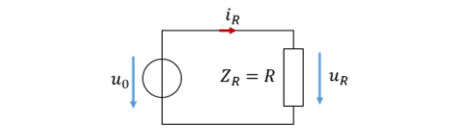
\[ \begin{gathered} \text{Source voltage: } u_0(t) = 3\,\mathrm{V} \cdot \sin(\omega t) \text{ with } \varphi_{u0} = 0 \\[4pt] u_0(\omega) = 3\,\mathrm{V} \text{ with } \varphi_{u0} = 0 \\[4pt] \text{Mesh equation: } u_R(\omega) = u_0(\omega) \\[4pt] \text{Impedance of the resistor: } Z_R = R = 6\,\Omega \\[4pt] \text{Current: } i_R(\omega) = \frac{u_R(\omega)}{Z_R} = \frac{3\,\mathrm{V}}{6\,\Omega} = 0.5\,\mathrm{A} \text{ with } \varphi_{iR} = 0 \end{gathered} \]

Simulation

In the figure below, you see at the top the time curve of voltage and current at the resistor. It becomes clear that there is no phase shift. Below that, you see the complex voltage and the complex current. They are not plotted over time t, but over the angular frequency ω. In this representation, current and voltage are points. At the very bottom, you see the phase of current and voltage plotted over the angular frequency ω. The phase is also a point in the diagram in each case.

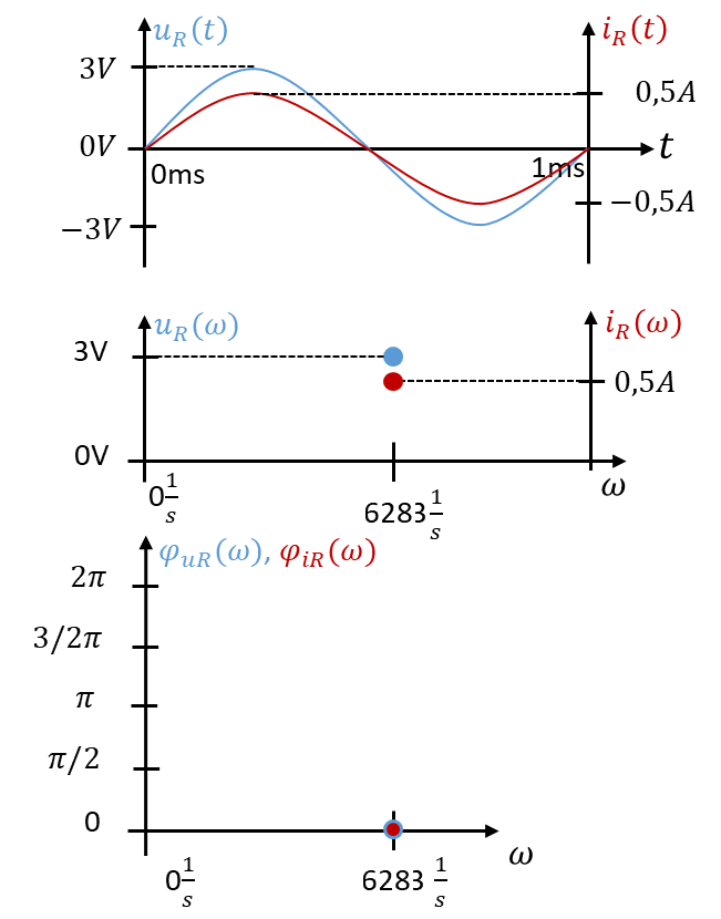
Voltage and current at the resistor in the time domain, and peak values and phases over the angular frequency ω

In the upper figure, the curves of voltage and current are shown simultaneously in one graph. Since current and voltage are on different y-axes with different units, a separate y-axis must be drawn for each. The red current curves therefore apply to the current axis, the blue voltage curves to the voltage axis. The x-axis (time axis) applies to both curves. In the bottom graph, the phases for voltage and current are the same. So that both can be seen, the point of the current phase is shown somewhat smaller than that of the voltage phase.

Capacitor

We now apply the same voltage u₀ to a capacitor with C = 1 mF. First we calculate the impedance of the capacitor. For this, the frequency f is important. In the example, we operate the circuit at f = 1 kHz. The following applies

\[ \begin{gathered} f = 1\,\mathrm{kHz} \rightarrow T = \frac{1}{f} = 1\,\mathrm{ms} \\[4pt] \omega = 2\pi f = 6.28\,\mathrm{k}\frac{1}{\mathrm{s}} \\[4pt] Z_C = \frac{1}{j\omega C} = \frac{1}{j6.28\,\mathrm{k}\frac{1}{\mathrm{s}} \cdot 1\,\mathrm{mF}} = -j160\,\mathrm{m\Omega} = 160\,\mathrm{m\Omega} \cdot e^{-j\frac{\pi}{2}} \end{gathered} \]

As a reminder: 1/j = −j. Since an impedance always represents the quotient of voltage and current, every impedance must have the unit Ω. The imaginary part of the impedance of a capacitor is always negative. For the current, the following applies:

\[ \begin{gathered} \text{Mesh equation: } u_C(\omega) = u_0(\omega) = 3\,\mathrm{V} \text{ with } \varphi_{uC} = 0 \\[4pt] i_C(\omega) = \frac{u_C(\omega)}{Z_C} = \frac{3\,\mathrm{V}}{160\,\mathrm{m\Omega} \cdot e^{-j\frac{\pi}{2}}} = \frac{3\,\mathrm{V}}{160\,\mathrm{m\Omega}} \cdot e^{j\frac{\pi}{2}} = j18.85\,\mathrm{A} \text{ with } \varphi_{iC} = \frac{\pi}{2} \\[6pt] \text{Alternatively: } i_C(\omega) = \frac{u_C(\omega)}{Z_C} = \frac{3\,\mathrm{V}}{(-j) \cdot 160\,\mathrm{m\Omega}} = j \cdot \frac{3\,\mathrm{V}}{160\,\mathrm{m\Omega}} = j18.85\,\mathrm{A} \end{gathered} \]

Simulation

In the time curve, the current is shifted to the left by π/2 relative to the voltage. The current leads the voltage. The peak value of the current is 18.85 A. It depends on the term ωC of the impedance. So the peak value of the current at the capacitor is also a function of frequency. The current increases linearly with increasing frequency.

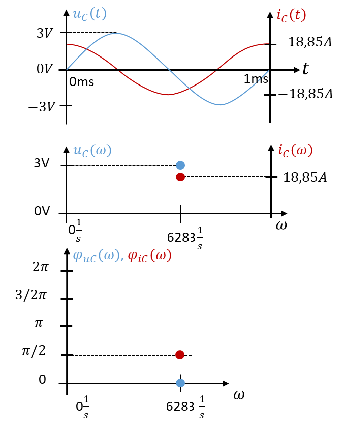
Voltage and current at the capacitor in the time domain, and peak values and phases over the angular frequency ω

The parameters j and ω are used to calculate the capacitor impedance. The angular frequency ω enters the numerical value of the impedance and is then no longer visible in the formulas. The parameter j is carried along in the further calculations.

Inductor

We now operate the source on an inductor. Next, let us calculate the impedance of an inductor with L = 5 mH. Then we calculate the associated current from voltage and impedance:

\[ \begin{gathered} Z_L = j\omega L = j6.28\,\mathrm{k}\frac{1}{\mathrm{s}} \cdot 5\,\mathrm{mH} = j31.4\,\Omega = 31.4\,\Omega \cdot e^{j\frac{\pi}{2}} \\[4pt] \text{Mesh equation: } u_L(\omega) = u_0(\omega) = 3\,\mathrm{V} \text{ with } \varphi_{uL} = 0 \\[4pt] i_L(\omega) = \frac{u_L(\omega)}{Z_L} = \frac{3\,\mathrm{V}}{31.4\,\Omega \cdot e^{j\frac{\pi}{2}}} = \frac{3\,\mathrm{V}}{31.4\,\Omega} \cdot e^{-j\frac{\pi}{2}} = 96\,\mathrm{mA} \cdot e^{-j\frac{\pi}{2}} = -j96\,\mathrm{mA} \text{ with } \varphi_{iL} = -\frac{\pi}{2} \\[6pt] \text{Alternatively: } i_L(\omega) = \frac{u_L(\omega)}{Z_L} = \frac{3\,\mathrm{V}}{j31.4\,\Omega} = -j\frac{3\,\mathrm{V}}{31.4\,\Omega} = -j96\,\mathrm{mA} \end{gathered} \]

Simulation

Voltage and current at the inductor in the time domain, and peak values and phases over the angular frequency ω — entspricht = corresponds to

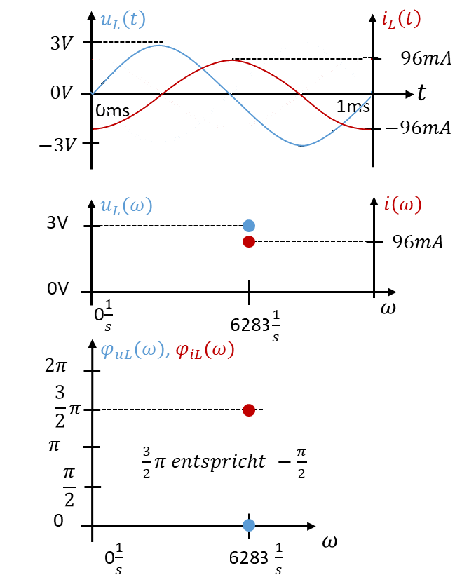
At the inductor, too, the current depends on the frequency. At constant voltage, it decreases with increasing frequency f.