Control Engineering › Oscillating Systems 2

Systems Capable of Oscillation

Systems capable of oscillation with two storage elements and at least one limiting element are called PT2 systems. In general, these systems have the following transfer function:

\[ \begin{gathered} \text{General PT2 transfer function:} \\[6pt] H_{\mathrm{PT2}}(s) = \frac{k_{P,\mathrm{PT2}}}{\frac{1}{\omega_0^2} s^2 + \frac{2D}{\omega_0} s + 1} \end{gathered} \]

The parameter k_P,PT2 in the numerator indicates the static gain of the system. The denominator contains the parameters resonant frequency “ω₀” and damping “D”. In the frequency domain, the complex frequency s is always the variable quantity. In the steady state at s = 0:

\[ \begin{gathered} \text{Steady state: } s = 0 \\[6pt] H_{\mathrm{PT2}}(0) = \frac{k_{P,\mathrm{PT2}}}{\frac{1}{\omega_0^2} 0^2 + \frac{2D}{\omega_0} 0 + 1} = k_{P,\mathrm{PT2}} \end{gathered} \]

Systems with PT2 behaviour may or may not oscillate. The damping and resonant frequency of these systems depend on the parameter settings of the function blocks. Via the controller settings, we can generally influence damping and resonant frequency.

The following cases are distinguished for the damping:

D = 0: continuous undamped oscillation

0 < D < 1: decaying oscillation

D = 1: critical damping: just no oscillation

D > 1: non-oscillating system

To analyse a PT2 system, we compare coefficients. We set the general equation of the behaviour equal to the specific equation of the system under consideration. I show this with the following example. We take a system with PT1 behaviour and I behaviour connected in series in a control loop. So parameter A consists of I behaviour and PT1 behaviour. For simplicity, we set τ of the system to 1:

Control loop with controller k_I, integrator 1/s and PT1 element 1/(1 + s)

\[ \begin{gathered} A = k_I \cdot \frac{1}{s} \cdot \frac{1}{1 + s} = \frac{k_I}{s + s^2} \\[6pt] \frac{1}{A} = \frac{s + s^2}{k_I} \\[6pt] H_{\mathrm{FÜ}}(s) = \frac{1}{1 + \frac{1}{A}} = \frac{1}{1 + \frac{s + s^2}{k_I}} = \frac{1}{\frac{1}{k_I} s^2 + \frac{1}{k_I} s + 1} \\[6pt] H_{\mathrm{PT2}}(s) = \frac{k_{P,\mathrm{PT2}}}{\frac{1}{\omega_0^2} s^2 + \frac{2D}{\omega_0} s + 1} \\[6pt] H_{\mathrm{FÜ}} = H_{\mathrm{PT2}} = \frac{1}{\textcolor{#c0392b}{\frac{1}{k_I}} s^2 + \textcolor{#2e75b6}{\frac{1}{k_I}} s + 1} = \frac{k_{P,\mathrm{PT2}}}{\textcolor{#c0392b}{\frac{1}{\omega_0^2}} s^2 + \textcolor{#2e75b6}{\frac{2D}{\omega_0}} s + 1} \\[6pt] \text{Comparing coefficients:} \\[6pt] \text{Numerator: } k_{P,\mathrm{PT2}} = 1 \\[6pt] \text{Denominator, before } s^2\text{: } \textcolor{#c0392b}{\frac{1}{\omega_0^2} = \frac{1}{k_I}} \rightarrow \omega_0 = \sqrt{k_I} \\[6pt] \text{Denominator, before } s\text{: } \textcolor{#2e75b6}{\frac{1}{k_I} = \frac{2D}{\omega_0}} = \frac{2D}{\sqrt{k_I}} \rightarrow D = \frac{1}{2\sqrt{k_I}} \end{gathered} \]

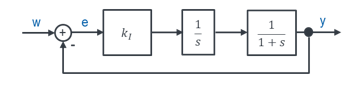
The parameter k_I together with the integrator 1/s represents the I behaviour. It is followed by a function block with PT1 behaviour, modelled in the example with k_P = 1 and τ = 1. The value of the damping D depends on the parameter k_I. So that the system oscillates “slightly”, we first set k_I = 10.

\[ \begin{gathered} D = \frac{1}{2\sqrt{k_I}} \\[6pt] \text{Set } k_I = 10 \\[6pt] D = \frac{1}{2\sqrt{10}} \approx 0.16 < 1 \end{gathered} \]

The damping D is less than 1, so the system oscillates. But it is greater than 0, so it does not oscillate permanently. It behaves like a swing that slows down because of friction. The step response shows typical oscillating PT2 behaviour with slight “overshoot”. The controlled variable overshoots the reference variable and then oscillates around the value of the reference variable. The oscillation decays, so that eventually the controlled variable reaches the value of the reference variable.

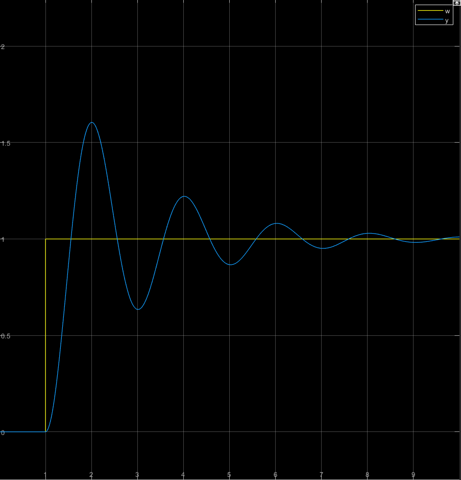
Simulated step response for k_I = 10: damped oscillation of y around the setpoint w = 1

The controlled variable reaches the reference variable for the first time after only about 0.5 s. That is quite fast compared with non-oscillating PT2 systems. The characteristic parameter ω₀ indicates the angular frequency of the decaying oscillation. We determine the oscillation angular frequency from the graph via the period. It is defined as the time between two maxima of the decaying oscillation.

\[ \begin{gathered} \text{Calculation: } \omega_0 = \sqrt{k_I} \\[6pt] \text{Set } k_I = 10 \rightarrow \omega_0 = \sqrt{10} \approx 3.16\,\frac{1}{\mathrm{s}} \\[6pt] \text{Reading between the maxima: } T_0 \approx 4\,\mathrm{s} - 2\,\mathrm{s} = 2\,\mathrm{s} \\[6pt] f_0 = \frac{1}{T_0} = 0.5\,\mathrm{Hz} \\[6pt] \omega_0 = 2\pi f_0 = 3.14\,\frac{1}{\mathrm{s}} \end{gathered} \]

The calculation agrees quite well with the value read off. The oscillation decays, so that after a long time we reach the steady state. Here y = 1 applies.

\[ \begin{gathered} \text{Steady state: } s = 0 \\[6pt] H_{\mathrm{FÜ}}(0) = \frac{1}{\frac{1}{k_I} 0^2 + \frac{1}{k_I} 0 + 1} = 1 \end{gathered} \]

We characterise the overshoot as follows: the maximum value of the controlled variable is about y = 1.6 at t = 2 s (seconds). The reference variable steps to w = 1. So the controlled variable overshoots the value of the reference variable by 60 %.

The damping D is difficult to read from the graph. There are formulas for this, but they are rather inaccurate and complex to calculate.

By changing the parameter k_I, we can change the behaviour of the system. With larger k_I, the damping decreases and the oscillation frequency increases. This is shown by the following simulation for k_I = 100:

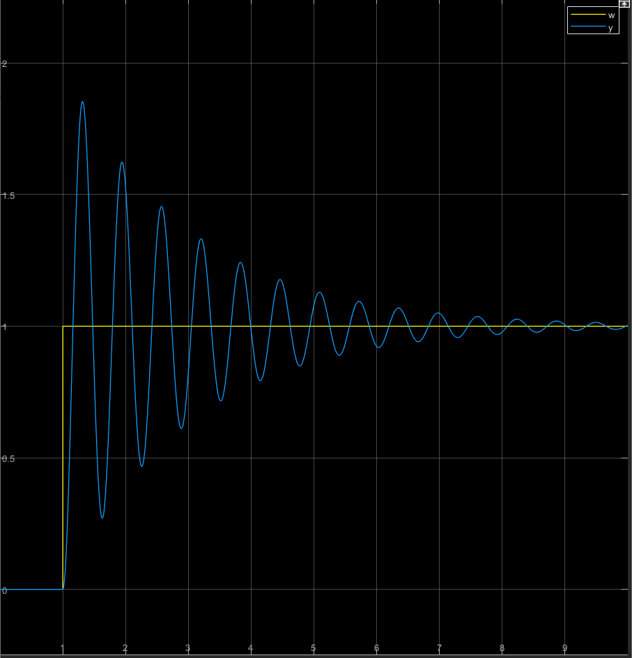
Simulated step response for k_I = 100: weakly damped, faster oscillation of y around the setpoint w = 1

\[ \begin{gathered} \text{Calculation: } \omega_0 = \sqrt{k_I} \\[6pt] \text{Set } k_I = 100 \rightarrow \omega_0 = \sqrt{100} = 10\,\frac{1}{\mathrm{s}} \\[6pt] \text{Reading between the maxima: } T_0 \approx 0.65\,\mathrm{s} \\[6pt] f_0 = \frac{1}{T_0} = 1.54\,\mathrm{Hz} \\[6pt] \omega_0 = 2\pi f_0 = 9.67\,\frac{1}{\mathrm{s}} \\[6pt] D = \frac{1}{2\sqrt{100}} = \frac{1}{20} = 0.05 \end{gathered} \]

The controlled variable reaches the reference variable for the first time after only about 0.2 s. Because of the lower damping of D = 0.05, the overshoot increases to about 85 %. The resonant frequency has become larger.

Critical damping with D = 1 is often aimed for, because it represents the fastest possible rise of the controlled variable without overshoot. In the example system we need

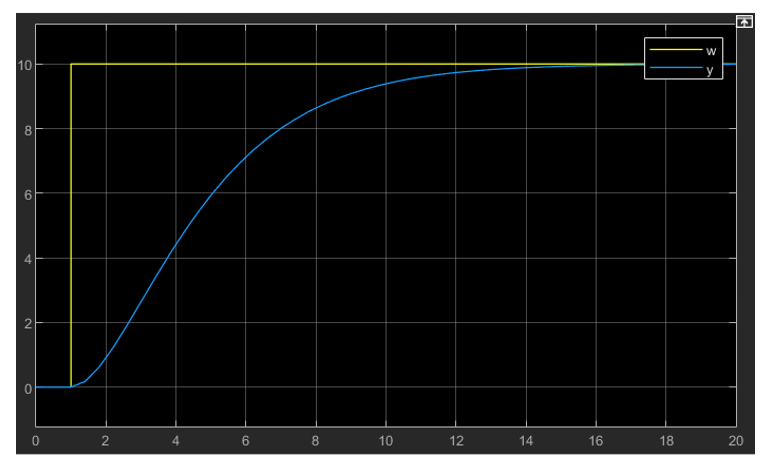
\[ D = \frac{1}{2\sqrt{k_I}} = 1\text{: } k_I = 0.25 \rightarrow D = \frac{1}{2\sqrt{0.25}} = 1 \]

Simulated step response with critical damping D = 1: y approaches the setpoint w without overshoot

In the step response, the simulation time has been doubled to 20 s so that the settling can still be shown. The time until the system reaches its steady state has become considerably longer with greater damping (D = 1 instead of D = 0.16). In return, the controlled variable does not overshoot.

Effects of overshoot

With overshoot, the controlled variable exceeds the maximum intended value. Overshoot is often problematic in control loops, because components are briefly loaded more heavily than planned. This can damage the components.

In a pressure control loop, for example, there is a maximum target pressure of 10 bar. But if the controlled system overshoots by 80 %, pressures of 18 bar can occur briefly. The components must be able to withstand that. This overdimensioning costs money.

Parameter optimisation

Let us compare the three cases considered so far. With critical damping D = 1, the output quantity is sluggish. It takes a long time to reach the value of the reference variable. In return, the controlled variable does not overshoot.

With k_I = 10, D = 0.16 applies. The controlled variable overshoots by about 60 %. In return, the controlled variable reaches the final value faster. With k_I = 100 and D = 0.05, the controlled variable overshoots by about 85 %. In return, it reaches the value of the reference variable even faster.

The larger the gain chosen in a control loop with 2 storage elements, the faster the controlled variable reaches the value of the reference variable. The resonant frequency becomes larger. The controlled variable overshoots more. Here we have to find a compromise for the application. We cannot achieve everything at the same time. A system without overshoot is slower than it could be.

A sluggish system reacts slowly to changes. During the transition time until the steady state is reached, the controlled variable sometimes deviates considerably from the reference variable. If sluggishness and temporary control errors are not a problem for the application, you should set critical damping D = 1 on the controller.

One example is the cruise control in a car. It is fine if it takes a few seconds for the speed to adjust to a new desired speed. On the other hand, it would be quite annoying if the speed briefly overshot the setpoint by 50 %. That is why critical damping is aimed for here.

For a machine tool, the world does not end if the speed of a drill is 50 % too high for a moment. But it depends on being able to change the speed very quickly. If the machine is to drill 100 holes per minute into the boards of an Ikea cupboard, the drill must react pretty quickly. Here one would set D between 0 and 1 so that the settling time is short.

Extending the goals

For a control loop, the goals are extended as follows:

1. H_FÜ = 1 should apply.

2. The system should settle in the shortest possible time, i.e. reach its final value.

3. The overshoot should be limited to a maximum value. The system should not oscillate permanently.