Control Engineering › System Behaviors 2

Dead Time

A system whose output reacts to the input in a step response only with a time delay has a dead time. A system with PT1 behaviour also has a time delay, but in addition an exponential transient behaviour. Dead time is exclusively a time shift in the output signal.

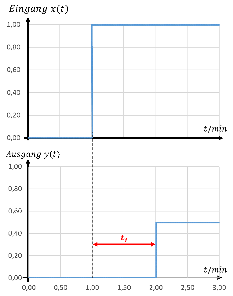
We consider two points in time: at time t₁ the input quantity steps. At time t₂ the output quantity shows the first reaction to the step. The dead time is then t_T = t₂ − t₁.

A practical example is a conveyor belt. At the input, an object is placed on the belt. The object reaches the output with a time delay.

Dead times exist in addition to all other behaviours. A P system with k_P = 0.5 and t_T = 1 min, for example, shows the following step response:

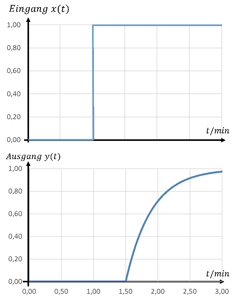
Step at input x(t) at t = 1 min and step at output y(t) delayed by the dead time t_T — Eingang = input · Ausgang = output

A system with PT1 behaviour and the parameters k_P = 2, τ = 0.75 min and t_T = 0.5 min shows the following step response:

Step at input x(t) at t = 1 min and PT1 response at output y(t) that only begins after a dead time at t = 1.5 min — Eingang = input · Ausgang = output

Dead time is not calculated in this tutorial. The mathematics is dreadful. You only need to know the effect and be able to determine a dead time in a step response.