Control Engineering › Controlled Systems

Example Control Loop

The general solution of all control loops from the last chapter can be used for any concrete control loop. To do this, you only have to substitute the product of the transfer functions of controller, actuator and plant for the general parameter A. We continue to use only blocks with P behaviour. For the general control loop:

\[ A = H_{\mathrm{Regler}} \cdot H_{\mathrm{Aktor}} \cdot H_{\mathrm{Strecke}} \]

Example: speed control

A machine tool should turn a drill at the output at a speed of 100 rpm. The machine consists of a motor and a gearbox. It is integrated into the following control loop:

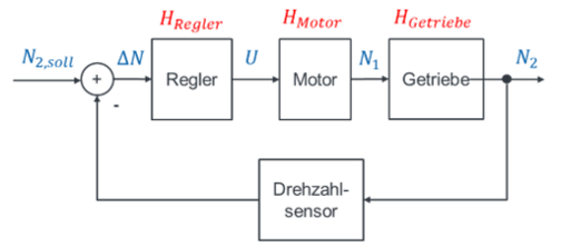
Speed control: controller, motor, gearbox and speed sensor in the control loop — Getriebe = gearbox · Regler = controller · Drehzahlsensor = speed sensor

\[ \begin{gathered} H_{\mathrm{Regler}}\text{: value set later, unit } \frac{\mathrm{V}}{\mathrm{rpm}} \\[6pt] \text{Example: } H_{\mathrm{Motor}} = 2\,\frac{\mathrm{rpm}}{\mathrm{V}} \\[6pt] H_{\mathrm{Getriebe}} = 5\,\frac{\mathrm{rpm}}{\mathrm{rpm}} \\[6pt] H_{\mathrm{Drehzahlsensor}} = 1 \end{gathered} \]

(Regler = controller, Getriebe = gearbox, Drehzahlsensor = speed sensor.) Let us first look at the transfer functions of the function blocks. They are given, for example, on the rating plates of the components. Alternatively, we can determine them with a step response. To do so, we have to measure the components individually, without them being installed in the control loop.

However we determined the transfer functions, we now use them to design the controller. We initially set the controller to H_R = 1 V/rpm; we will optimise it later. So for A in the specific control loop:

Simplified control loop of the speed control with w = N2,soll and y = N2 — Soll = setpoint

\[ \begin{gathered} \text{Reference variable } w = N_{2,\mathrm{soll}} \text{ (target output speed)} \\[6pt] \text{Controlled variable } y = N_2 \text{ (output speed)} \\[6pt] A = H_{\mathrm{Regler}} \cdot H_{\mathrm{Aktor}} \cdot H_{\mathrm{Strecke}} = 1\,\frac{\mathrm{V}}{\mathrm{rpm}} \cdot 2\,\frac{\mathrm{rpm}}{\mathrm{V}} \cdot 5\,\frac{\mathrm{rpm}}{\mathrm{rpm}} = 10 \\[6pt] \text{General: } y = \frac{A}{1 + A} \cdot w;\ \text{goal } y = w \\[6pt] \text{Speed control: } N_2 = \frac{A}{1 + A} \cdot N_{2,\mathrm{soll}};\ \text{goal } N_2 = N_{2,\mathrm{soll}} \\[6pt] \text{with } A = 10\text{:} \\[6pt] N_2 = \frac{10}{1 + 10} \cdot N_{2,\mathrm{soll}} = \frac{10}{11} \cdot N_{2,\mathrm{soll}} = 0.91 \cdot N_{2,\mathrm{soll}} \\[6pt] \text{Control error: } e = (1 - 0.91) \cdot N_{2,\mathrm{soll}} = 0.09 \cdot N_{2,\mathrm{soll}} \end{gathered} \]

Note: because w and y always have the same units, A is always dimensionless.

With A = 10 the control is rather poor, because the control error e is 9 %. If we specify a desired speed of N_2,soll = 1000 rpm, the output shaft only turns at 910 rpm. So far we have not optimised the controller. We can, for example, set the controller value to 100 V/rpm, which increases A to 1000. Then:

\[ \begin{gathered} H_{\mathrm{Regler}} = 100\,\frac{\mathrm{V}}{\mathrm{rpm}} \rightarrow A = 1000 \\[6pt] N_2 = \frac{1000}{1 + 1000} \cdot N_{2,\mathrm{soll}} = \frac{1000}{1001} \cdot N_{2,\mathrm{soll}} = 0.999 \cdot N_{2,\mathrm{soll}} \\[6pt] e = (1 - 0.999) \cdot N_{2,\mathrm{soll}} = 0.001 \cdot N_{2,\mathrm{soll}} \end{gathered} \]

The control error is now only 0.1 % of the setpoint. The output shaft now turns at 999 rpm when we specify 1000 rpm. That is already much better. With the controller, we optimise A as we need it.

What is the point? What is it good for?

Perhaps at this point you are asking yourself what all this is good for ;-). Why do we use something as complicated as a control loop just so that a speed is set correctly at the output? There are three good reasons:

1. We only look at disturbances much later in the tutorial. A preview: whatever disturbances occur in the system, this control loop always keeps the output speed at the setpoint, no matter what happens.

2. The control loop does this autonomously, without anyone having to intervene from outside. You leave the machine tool alone, and it keeps turning at the target speed. When a workpiece is to be machined, the machine is braked. The control loop ensures that this has (ideally) no influence on the speed.

3. For closed-loop control, we do not need to understand the internal structure and the internal mathematics of a system. Feel free to look again at the introductory chapters on the difference between open-loop and closed-loop control.