PID Controller

In practice you mainly encounter PID controllers. With these controllers you can set the behaviours P, I and D with different intensities. You can, for example, give a controller mainly P behaviour and a little I behaviour. This type of controller is an industry standard. Almost all methods for controller design refer to PID controllers.

PT1 controllers are practically never used. They would only be slower P controllers with an additional storage element in the system. Pure P behaviour is generally better than PT1 behaviour in a controller.

The disadvantage of these controllers is the complexity of their behaviour in a controlled system. If you use PID controllers, you often can no longer calculate the behaviour of the controlled system by hand. You then switch completely to simulation. For the design, however, it is important to understand how the behaviours P, I and D generally act on systems. We discussed this in detail in the last chapters. If you are still unsure about it, please revise it now.

A PID controller has the following structure:

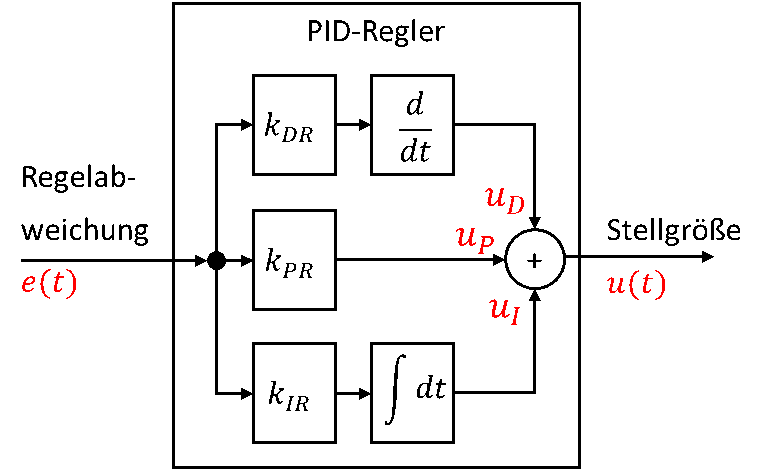
PID controller in the time domain: parallel connection of D component (k_DR, d/dt), P component (k_PR) and I component (k_IR, integral) from e(t) to u(t) — PID-Regler = PID controller · Regelabweichung = control error · Stellgröße = manipulated variable

The control error is the input quantity of every controller. It is differentiated (D), integrated (I) and amplified (P). Each component is multiplied by an adjustable controller parameter. Before we start calculating, we switch to the frequency domain again:

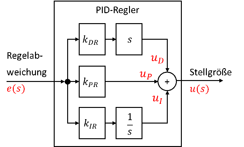
PID controller in the frequency domain: parallel connection of D component (k_DR, s), P component (k_PR) and I component (k_IR, 1/s) from e(s) to u(s) — PID-Regler = PID controller · Regelabweichung = control error · Stellgröße = manipulated variable

Multiplication by s corresponds to differentiation and division by s corresponds to integration. The following equations apply:

\[ \begin{gathered} u_D = k_{DR} \cdot s \cdot e \\[6pt] u_P = k_{PR} \cdot e \\[6pt] u_I = k_{IR} \cdot \frac{1}{s} \cdot e \\[6pt] u = u_D + u_P + u_I \\[6pt] u = \left(k_{DR} \cdot s + k_{PR} + k_{IR} \cdot \frac{1}{s}\right) \cdot e \\[6pt] H_R = \frac{u}{e} = k_{DR} \cdot s + k_{PR} + k_{IR} \cdot \frac{1}{s} \end{gathered} \]

The intensity of the individual behaviours is specified by the three controller parameters k_DR, k_PR and k_IR, which you as the developer set in the controller software.

You build a pure I controller, for example, by setting k_PR and k_DR to 0. PI controllers are frequently used, in which only k_DR = 0 applies.

Controlled systems

To calculate the reference response of a system controlled with a PID controller, we use H_S in general as the transfer function of the system. Then:

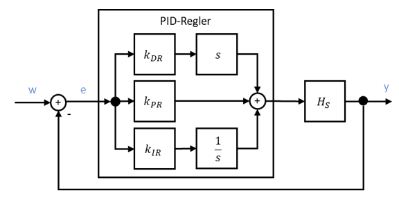
Control loop with PID controller and plant H_S — PID-Regler = PID controller

\[ \begin{gathered} A = H_S \cdot \left(k_{DR} \cdot s + k_{PR} + k_{IR} \cdot \frac{1}{s}\right) \\[6pt] H_{\mathrm{FÜ}} = \frac{A}{1 + A} = \frac{H_S \cdot \left(k_{DR} \cdot s + k_{PR} + k_{IR} \cdot \frac{1}{s}\right)}{1 + H_S \cdot \left(k_{DR} \cdot s + k_{PR} + k_{IR} \cdot \frac{1}{s}\right)} \end{gathered} \]

The transfer function of the controlled system is too complicated for calculations by hand, especially when a transfer function of the system is added. This example only serves as a deterrent, so that you do not get the idea of calculating something like this. We do not do it in the exam either.

Alternative representation and calculation

In practice, PID controllers are often represented and calculated differently. The following alternative representation is widespread:

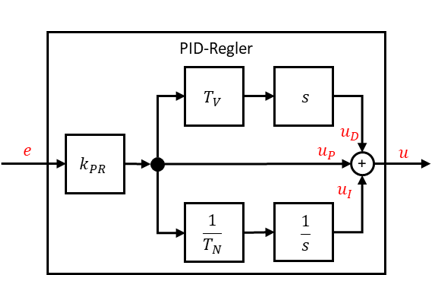
PID controller with upstream k_PR, derivative time T_V and reset (integral) time T_N — PID-Regler = PID controller

\[ \begin{gathered} u_D = k_{PR} \cdot T_V \cdot s \cdot e \\[6pt] u_P = k_{PR} \cdot e \\[6pt] u_I = k_{PR} \cdot \frac{1}{T_N} \cdot \frac{1}{s} \cdot e \\[6pt] u = u_D + u_P + u_I \\[6pt] u = k_{PR} \cdot T_V \cdot s \cdot e + k_{PR} \cdot e + k_{PR} \cdot \frac{1}{T_N} \cdot \frac{1}{s} \cdot e \\[6pt] u = k_{PR} \cdot \left(T_V \cdot s + 1 + \frac{1}{T_N} \cdot \frac{1}{s}\right) \cdot e \\[6pt] H = \frac{u}{e} = k_{PR} \cdot \left(T_V \cdot s + 1 + \frac{1}{T_N} \cdot \frac{1}{s}\right) \end{gathered} \]

(T_V = derivative time, T_N = reset or integral time.) If you (have to) use a controller with the alternative parameters, you can convert the parameters as follows:

\[ \begin{gathered} k_{DR} = k_{PR} \cdot T_V \\[6pt] T_V = \frac{k_{DR}}{k_{PR}} \\[6pt] k_{IR} = k_{PR} \cdot \frac{1}{T_N} \\[6pt] T_N = \frac{k_{PR}}{k_{IR}} \end{gathered} \]

The setting options remain the same with the alternative representation. However, the parameter k_PR also acts on the D and I behaviour of the controller. You can enter the parameters T_V and T_N directly into the controller software, just as you would otherwise enter k_DR and k_IR. I prefer the parameterisation shown further above, because it allows the three behaviours to be set independently of each other.