Control Engineering › Controlled Systems

Proportional Behavior

Similarity

Many real technical systems behave similarly. We describe similar systems with the same formula, into which we insert different parameters. One example is the straight-line equation. You can use it to calculate very different systems. For each, you insert suitable parameters m and b. In general, for all linear systems:

\[ \begin{gathered} \text{General straight-line equation: } y = m \cdot x + b \\[6pt] \text{Specific parameters in an example: } m = 1 \text{ and } b = 5 \\[6pt] \text{Specific straight-line equation: } y = x + 5 \end{gathered} \]

Which systems can be calculated with the straight-line equation? Well, all linear systems, because the straight-line equation is linear. In this chapter, in addition to linearity, we look for further system properties that characterise their behaviour. For each, there is a general formula for calculating all systems with this behaviour. The general formula has characteristic parameters with which you adapt it to your problem.

Transfer function

The transfer function indicates how an input quantity is changed by a system or a function block. The output quantity is generally different from the input quantity. The transfer function H describes the change of the input quantity mathematically. From H we recognise the type of behaviour of the system.

Function block H with input and output — Eingang = input · Ausgang = output

\[ \begin{gathered} \text{General description of a function block or system:} \\[6pt] \text{Output} = H \cdot \text{input} \\[6pt] H = \frac{\text{output}}{\text{input}} \end{gathered} \]

Proportionality

We start with the simplest type of behaviour: proportional behaviour. In systems with proportional behaviour, the output quantity is proportional to the input quantity. In control engineering, proportional behaviour is abbreviated as “P behaviour”. With proportional behaviour, the transfer function H is a constant:

\[ \begin{gathered} \text{If } H \text{ is a constant} \rightarrow \text{proportional behaviour} \\[6pt] H = k_P \text{ with } k_P\text{: “proportional constant”} \\[6pt] \text{Output} = y \\[6pt] \text{Input} = x \\[6pt] y = k_P \cdot x \end{gathered} \]

In a control loop, we model a function block with P behaviour as a square with the label k_P in the centre. Instead of the label k_P, the numerical value of k_P can also be written there directly.

The equation between output and input of a system with proportional behaviour is a special case of the straight-line equation.

\[ \begin{gathered} \text{General straight-line equation: } y = m \cdot x + b \\[6pt] \text{Proportional behaviour: } y = m \cdot x \text{ with } b = 0 \\[6pt] H = m = k_P \end{gathered} \]

The slope m corresponds to the proportional constant k_P. A system whose input and output quantities satisfy a straight-line equation behaves linearly. Linear behaviour with b = 0 is called proportional behaviour. If input and output quantities are plotted against each other, the following picture results for, e.g., k_P = 3:

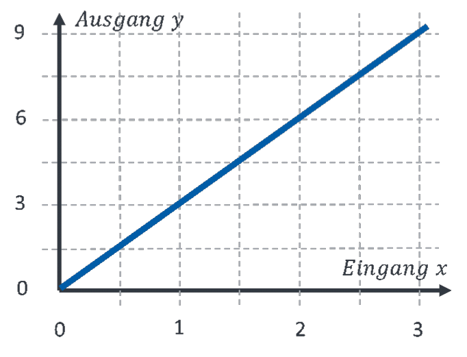
Proportional behaviour: output y rises linearly with input x (straight line through the origin) — Ausgang = output · Eingang = input

If the input is 0, the output is also 0. If the input quantity rises, the output quantity also rises. This is characteristic of proportional behaviour. With, e.g., k_P = 3, the output value is three times as large as the input value.

From the point of view of control engineering, a proportional system is fully described by the parameter k_P. If you model a system with P behaviour, you define its input quantity x(t) and its output quantity y(t). The parameter k_P corresponds to the quotient of output quantity y divided by input quantity x. So k_P corresponds to the transfer function H.

\[ \begin{gathered} y = k_P \cdot x \\[6pt] \text{Determining } k_P\text{: determine one pair of values } x_1 \text{ and } y_1 \\[6pt] k_P = H = \frac{y_1}{x_1} \end{gathered} \]

After the general definition, let us look at a few examples.

Example: resistor

The relationship between voltage and current at a resistor in electrical engineering is proportional. If we define the voltage as the output and the current as the input of the function block resistor, the resistance R forms the proportional constant.

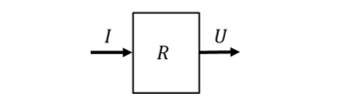
\[ \begin{gathered} \text{General: output} = k_P \cdot \text{input} \\[6pt] \text{Example: } U = R \cdot I \\[6pt] \text{with } H = k_P = R \end{gathered} \]

How do we determine k_P or R for the resistor? By measuring the current at any voltage. We insert these values into the general equation and obtain the specific value of our resistor R.

Example: gearbox

A gearbox also behaves proportionally. The input of the gearbox is the rotational speed N₁ at shaft 1 and the output is the rotational speed N₂ at shaft 2.

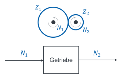
Gearbox with gears Z1 and Z2 as a block from N1 to N2 — Getriebe = gearbox

\[ \begin{gathered} \text{Input: } N_1;\ \text{output: } N_2 \\[6pt] N_2 = \frac{Z_1}{Z_2} \cdot N_1 \\[6pt] H = \frac{Z_1}{Z_2} = k_P \end{gathered} \]

If shaft 1 in the gearbox does not turn (input quantity = 0), shaft 2 does not turn either (output quantity = 0). The faster shaft 1 turns, the faster shaft 2 turns. How do we determine k_P? Either we count the teeth of the gears involved; then we determine k_P from the internal structure of the gearbox. Or we turn the input and measure the speed at the output; then we determine k_P from outside, without having to look inside the gearbox.

Example: lever

Another proportional system is the lever. The input and output quantities are the heights of the end points of the lever. If the height h₁ is changed as the input, the height h₂ also changes as the output. The lengths of the two arms of the lever determine the slope m or the transfer function H of the system.

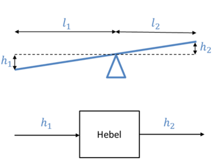
Lever with lengths l1 and l2 as a block from h1 to h2 — Hebel = lever

\[ \begin{gathered} h_2 = \frac{l_2}{l_1} \cdot h_1 \\[6pt] H = k_P = \frac{l_2}{l_1} \end{gathered} \]

Suppose, for example, the lengths are l₁ = 40 cm and l₂ = 30 cm; then this system can be described with H = k_P = 30 cm / 40 cm = 0.75. If the input moves from h₁ = 0 cm to h₁ = 10 cm, the output follows from h₂ = 0 cm to h₂ = k_P ∙ 10 cm = 7.5 cm.

Exploiting the similarity

Resistor, lever and gearbox behave similarly. All three systems can be calculated with the same mathematics. So they are treated in the same way in control engineering.

We first invest in a general solution for all systems with P behaviour. The general solution contains the characteristic parameter k_P.

Then we look at the specific system and define its input and output quantities. The characteristic parameter k_P is determined for the specific system, either by measuring input and output or from internal quantities. With input quantity, output quantity and characteristic parameter, we have transferred the general solution to a specific solution of a concrete problem.

Interpretation of k_P

An input signal is amplified by k_P by a function block with P behaviour. The gain of a signal can be greater than 1. Then the value of the output signal is larger than that of the input signal. The gain of a signal can be equal to 1. Then the signal is not changed by the block; its value at the output equals that at the input.

The gain of a signal can lie between 0 and 1. Then the signal is attenuated; its value at the output is smaller than at the input. If the gain is 0, no signal is output. If the gain is less than 0, the signal is inverted; its sign then changes in addition to its numerical value. The value of k_P generally has a unit, unless input and output quantities happen to have the same unit.

\[ \begin{gathered} |k_P| > 1\text{: amplification} \\[6pt] k_P = 1\text{: no change in signal} \\[6pt] 0 < |k_P| < 1\text{: attenuation} \\[6pt] k_P = 0\text{: output signal} = 0 \\[6pt] k_P < 0\text{: additional inversion} \end{gathered} \]