Average and RMS Value

When you operate a hair dryer at a mains socket, the question arises as to how much electrical energy is converted into thermal energy for the heat and kinetic energy for the air movement. With direct current, we can simply give the power as the product of current and voltage. With alternating current at a mains socket, it is not that simple. The question arises: what power is present on average over time? Which parameter do we give for this? The peak value is not suitable, because it is only present briefly twice per period. We do not have any other parameters yet.

In mathematics, we use the mean value for such information. The mean value of a quantity over time indicates how much of the quantity was present on average over a certain time. The mean value is the area under the curve divided by the time considered. The mean value of a quantity is marked with a horizontal bar above the quantity.

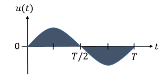
With sinusoidal quantities, we have the problem that the mean value over one sine period is always 0.

\[ \begin{gathered} \text{In general: } \overline{u} = \frac{1}{T} \int u(t)\,dt \\[4pt] \text{For a sinusoidal voltage with } u(t) = \hat{u} \cdot \sin(\omega t)\text{:} \\[4pt] \overline{u} = \frac{1}{T} \int_0^T \hat{u} \sin(\omega t)\,dt = -\frac{\hat{u}}{\omega T} \cos(\omega t)\Big|_0^T = -\frac{\hat{u}}{2\pi} \left(\cos(2\pi) - \cos(0)\right) = 0\,\mathrm{V} \end{gathered} \]

The area below the time axis and the area above it cancel each other out when the integral is summed. They are the same size but have different signs. This is shown by the following time curve of the voltage:

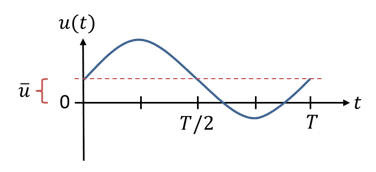
Sinusoidal voltage over one period: positive and negative half-waves are the same size

For symmetrical AC quantities, the mean value is 0. For certain AC quantities, it has a different meaning: if a curve is shifted along the y-axis, the mean value indicates by which value the curve is shifted. However, we do not yet consider such voltage and current curves in the fundamentals of electrical engineering. The following figure shows a voltage curve shifted upwards. The mean value gives the shift mathematically.

Sinusoidal voltage shifted upwards; the mean value ū indicates the shift

In electrical engineering, the mean value of a sinusoidal voltage is not used. So you do not need to be able to calculate it. We need a more suitable quantity to describe the area or “content” of a sinusoidal voltage.

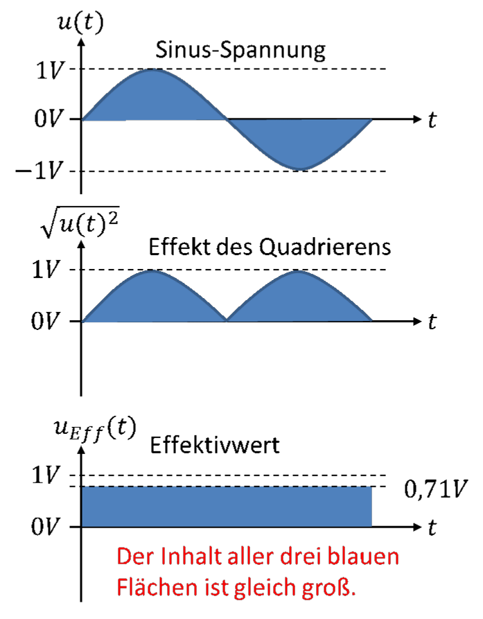
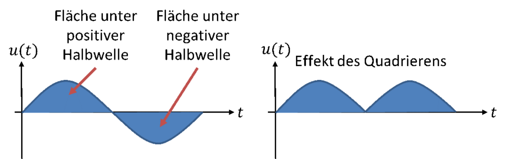
For the “content” of the sine function, we need a measure in which both area components are taken into account positively. If the function is first squared, then summed up and finally the square root is taken, we obtain a measure of the area of both components. Squaring makes the negative area component positive. By taking the square root, we mathematically compensate for the squaring. This is what the RMS value (root mean square, effective value) does.

Area under the positive and negative half-wave and the effect of squaring — Fläche unter positiver / negativer Halbwelle = area under the positive / negative half-wave · Effekt des Quadrierens = effect of squaring

The RMS value of the voltage u(t) is defined by the following formula:

\[ U_{\mathrm{eff}} = \sqrt{\frac{1}{T} \int_0^T u^2(t)\,dt} \]

If we substitute a sinusoidal voltage curve into the formula, the result is: the RMS value of a sinusoidal quantity equals the peak value divided by √2. The following applies:

\[ U_{\mathrm{eff}} = \sqrt{\frac{1}{T} \int_0^T \left(\hat{u} \cdot \sin(\omega t)\right)^2 dt} = \frac{\hat{u}}{\sqrt{2}} \]

So the RMS value is a measure of the magnitude of an area under a curve. In this tutorial (and also in the exam), we do not calculate the RMS value using the integral equation. We only consider RMS values of sinusoidal quantities, which can be calculated very easily with the simplification above.

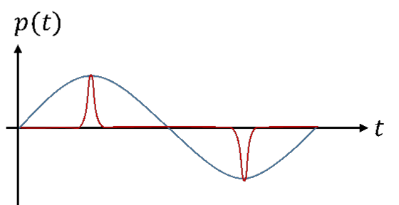
Can the “content” of a curve not be obtained more easily from other parameters? The following example shows that this does not work. The figure below shows two voltage curves over time. The classic parameters of the voltages are all the same: peak value, period and frequency. Only the red curve is not sinusoidal. Evidently, the areas under the curves are not the same size. If these were curves of the power over time of the hair dryer at the mains socket, the dryer would get properly hot with the blue curve, but only lukewarm with the red one. For the red curve, we would have to determine the RMS value from the integral, because the function is not a sine.

Two curves p(t) with the same peak value and the same period: sine (blue) and narrow pulses (red)

Remember: the RMS value is a quantity that is constant over time. Over one period, the square of the RMS value spans the same area with the x-axis as the square of the sine.

Sinusoidal voltage of 1 V, effect of squaring and RMS value 0.71 V: all three blue areas are the same size — Sinus-Spannung = sine voltage · Effekt des Quadrierens = effect of squaring · Effektivwert = RMS value · Der Inhalt aller drei blauen Flächen ist gleich groß = the three blue areas are equal in size