Control Engineering › System Behaviors 2

Control Loop Analysis

Let us look at the step response of a function block or of a characteristic system. In the last chapter we discussed that there are two characteristic points in time at which calculating the system is easy: after an infinitely long time, the system has settled after the step. The output quantity no longer changes over time. We calculate this behaviour by inserting s = 0 into the transfer function. This generally simplifies the transfer function considerably.

The second point is the step time. Here s → ∞ applies. This value of s is also generally easy to calculate. Let us look at PT1 behaviour again:

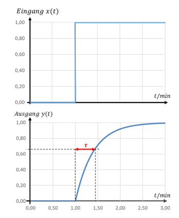
Step at input x(t) at t = 1 min and PT1 step response y(t) with time constant τ — Eingang = input · Ausgang = output

\[ \begin{gathered} \text{Step at the input from 0 to 1} \\[6pt] H_{\mathrm{PT1}}(s) = \frac{k_P}{1 + \tau \cdot s} \\[6pt] \text{Step time: } s \rightarrow \infty \\[6pt] H_{\mathrm{PT1}}(\infty) = \frac{k_P}{1 + \tau \cdot \infty} = 0 \\[6pt] \text{Steady state: } s = 0 \\[6pt] H_{\mathrm{PT1}}(0) = \frac{k_P}{1 + \tau \cdot 0} = k_P \end{gathered} \]

We do not consider the intermediate range mathematically, only phenomenologically. So we calculate nothing, but only look roughly at the transition range between the two states. I happily leave the calculation of the transition range to Matlab; that is not something you do by hand.

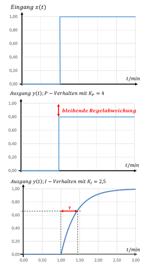
The quality of a control loop is assessed at the step time, in the transition range and in the steady state. At these three points, we compare the behaviours P and I in a control loop. To do so, we give A once only P behaviour and once I behaviour:

Step at the input and output y(t) for P behaviour (k_P = 4, steady-state error) and for I behaviour (k_I = 2.5) — Eingang = input · Ausgang = output · Verhalten = behaviour · Regelabweichung = control error · bleibende Regelabweichung = steady-state control error

\[ \begin{gathered} A = k_P\text{: P behaviour in the control loop: } H_{\mathrm{FÜ}} = \frac{k_P}{1 + k_P} \\[6pt] A = \frac{k_I}{s}\text{: I behaviour in the control loop: } H_{\mathrm{FÜ}} = \frac{1}{1 + \frac{1}{k_I} \cdot s} \end{gathered} \]

Step time

The step time indicates how the control loop reacts immediately to changes. P behaviour reacts at once. I behaviour reacts with a delay. We can read this directly from the step responses.

\[ \begin{gathered} \text{Step time with } s \rightarrow \infty\text{:} \\[6pt] A = \frac{k_I}{s}\text{: I behaviour in the control loop: } H_{\mathrm{FÜ}}(\infty) = \frac{1}{1 + \frac{1}{k_I} \cdot \infty} = 0 \\[6pt] A = k_P = 4\text{: P behaviour in the control loop: } H_{\mathrm{FÜ}}(\infty) = \frac{k_P}{1 + k_P} = \frac{4}{5} = 0.8 \end{gathered} \]

At the step time, the control loop with I behaviour does not react at all yet (H = 0). The control loop with P behaviour jumps directly to its final value (H = 0.8).

Transient behaviour

P behaviour has no transient behaviour, because it has no delaying effect. The transient behaviour of the control loop with I behaviour (PT1 reference response) is described by the parameter τ. The smaller τ is, the faster the output quantity reaches its final value.

Steady state

In the steady state, P behaviour has a steady-state control error. The output is y = 0.8 instead of y = 1 for k_P = 4. I behaviour, on the other hand, has no steady-state control error. With I behaviour, the output reaches the setpoint 1 completely.

\[ \begin{gathered} \text{Steady state with } s = 0\text{:} \\[6pt] A = \frac{k_I}{s}\text{: I behaviour in the control loop: } H_{\mathrm{FÜ}}(0) = \frac{1}{1 + \frac{1}{k_I} \cdot 0} = 1 \\[6pt] A = k_P = 4\text{: P behaviour in the control loop: } H_{\mathrm{FÜ}}(0) = \frac{k_P}{1 + k_P} = \frac{4}{5} = 0.8 \end{gathered} \]

Why does I behaviour have no steady-state control error? Let us compare the control loop with P behaviour and with I behaviour again:

\[ \begin{gathered} y = k_P \cdot e \\[6pt] e = \frac{1}{k_P} \cdot y \end{gathered} \]

Control loop with I element (k_I and 1/s)

\[ \begin{gathered} y = \frac{k_I}{s} \cdot e \\[6pt] e = \frac{s}{k_I} \cdot y \end{gathered} \]

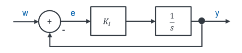
In a controlled system with P behaviour, e = 0 always means y = 0. That is why there must be a control error e if the system has a non-zero value at its output. Storage elements have the property that their output keeps its value constant when the input is 0. With a storage element we can therefore achieve e = 0 with y > 0. How does this work mathematically?

For H_FÜ = 1 we need A → ∞. In a system with P behaviour, the gain k_P must therefore be very large for the control error e to become small. When integrating, the output quantity keeps growing over time. In a system with I behaviour, we can therefore instead simply wait long enough.

Suppose that, in the control loop above with I behaviour, w = 1 and y = 0. Then e = w − y = 1. This is the inflow to the storage element. The fill level y rises over time. After some time, w = 1 and y = 0.5. Now e is only 0.5. The inflow to the storage element is smaller and the fill level y rises more slowly. But it still rises, so that somewhat later y = 0.9. Then e = 1 − 0.9 = 0.1. The control error e is now even smaller, so the storage element is filled ever more slowly.

Over time t, the control error e keeps decreasing, and the fill level y of the storage element approaches the setpoint w = 1 ever more closely. After a longer time, the control error is smaller than our measuring capabilities. We have reached the steady state. This explains the PT1-shaped settling process of the controlled system with I behaviour.

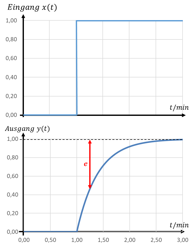
Step at input x(t) and output y(t) of an I control loop with the control error e marked — Eingang = input · Ausgang = output

In the graph, the control error e is shown as the difference between the line y = 1 and the curve of y(t). Of course this only applies after the step, from t ≥ 1 s. It becomes clear that e decreases over time and y approaches the setpoint ever more closely.