Oscillating Systems 1

Pendulum oscillation

One example of an oscillating system is a swing. After it has been pushed, a swing moves back and forth. A pendulum hanging on a string also swings back and forth. Another example is a weight hanging vertically from a coil spring. If you briefly pull the weight down from its rest position, it then oscillates up and down. In this tutorial we look at the pendulum as a relatively simple example. Please watch the following video:

Let us place the pendulum in a coordinate system so that we can describe its motion mathematically:

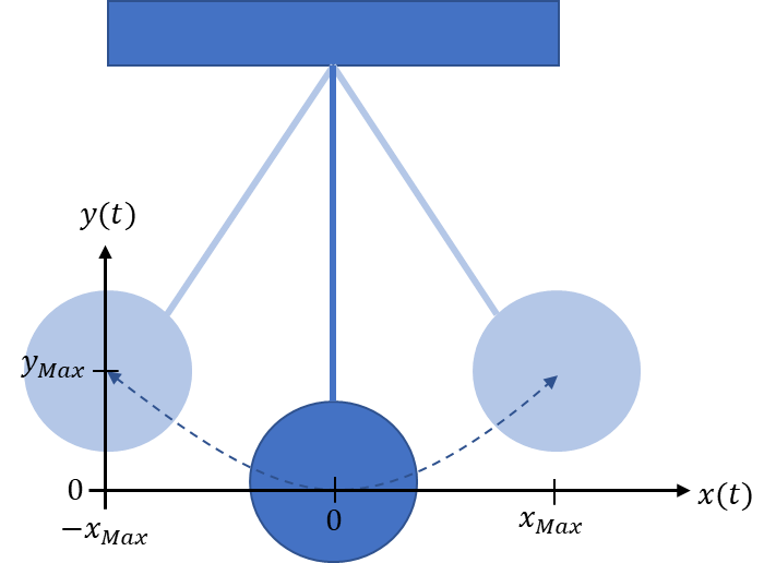
Pendulum with deflection between −x_Max and x_Max and height y up to y_Max

In dark blue you see the pendulum at rest. If we deflect the pendulum, e.g. to the left into the position shown in light blue, it then swings to the light blue position shown on the right and back again. The speed of the motion is v = 0 at the light blue end points. It is at its maximum at the dark blue starting position. The closer the pendulum gets to an end position, the slower the motion becomes.

A system can oscillate if energy can be exchanged between two coupled storage elements. If a system capable of oscillation is excited or pushed, it generally oscillates. Preventing the oscillation is harder than making the system oscillate, because oscillating is its “natural” behaviour.

Everything that moves outside a vacuum rubs against air or a surface. Real oscillations decay over time because, for example, friction slows down a motion. We first consider ideal oscillating systems that keep oscillating forever after being excited.

Mathematics of a pendulum oscillation

We look at the oscillation with as few formulas as possible. We plot what we observe in the video for the x-position and y-position over time. The motion of a swinging pendulum is sinusoidal.

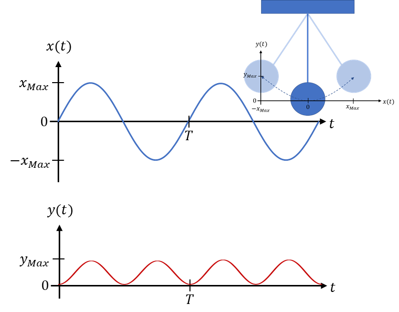
Time curves of the x-position (period T) and the y-position (twice the frequency) of the pendulum

The pendulum starts its motion at time t = 0 in the dark blue starting position. At the start, x = 0 and y = 0. It starts moving through an impulse from outside in the x direction, i.e. to the right. As a result, the y-position, i.e. its height, rises. After a quarter period, at t = T/4, it reaches its right end position with maximum height. It then moves to the left end position at t = 3T/4. Here too the y-position is maximally positive, but according to the chosen coordinate system the x-position is maximally negative. After one period of the oscillation, at t = T, the pendulum reaches the dark blue starting position again. The following formulas apply:

\[ \begin{gathered} x\text{-position: } x(t) = x_{\mathrm{max}} \cdot \sin(\omega t) \\[6pt] y\text{-position: } y(t) = \frac{1}{2} y_{\mathrm{max}} \cdot \bigl(1 - \cos(2\omega t)\bigr) \end{gathered} \]

If you have difficulties with the mathematics, it is enough to look at the time curves. The key relationships are also clear without formulas. The formulas only put them into a mathematical description that helps some people visualise them. So the formulas are not always helpful, and not for everyone.

The x-position is described by a sine containing the time t as a variable. After all, the position x(t) changes with time t. The y-position is shifted upwards by the peak value so that the shifted sine only has positive values. The frequency is twice that of the x-position. The sine is shifted to the right by π/2, so we can also write it as “−cos”. You do not need to be able to set up the formulas, but you should be able to understand from the time curves why they are valid.

In an oscillating system, energy is pushed back and forth between two energy storage elements. In the pendulum, the two forms of energy are potential energy (height) and kinetic energy (motion). Please watch the following video:

The following applies:

\[ \begin{gathered} \Delta W_{\mathrm{Pot}} = m \cdot g \cdot \Delta h = m \cdot g \cdot y = m \cdot g \cdot \frac{1}{2} y_{\mathrm{max}} \cdot \bigl(1 - \cos(2\omega t)\bigr) \\[6pt] \Delta W_{\mathrm{Pot}} = \frac{W_{\mathrm{Pot,max}}}{2} \cdot \bigl(1 - \cos(2\omega t)\bigr) \\[6pt] W_{\mathrm{Kin}} = \frac{1}{2} m \cdot v^2 \end{gathered} \]

We can calculate the potential energy from the y-position and the mass of the pendulum. Note: we only consider the change in potential energy ΔW_Pot. For this local experiment, we define the potential energy at the dark blue starting position as 0, although it lies far above the Earth’s core and is therefore of course not 0.

The speed of the pendulum is also sinusoidal. It is the time derivative of the position. For the speed we simplify the problem somewhat. We exploit the fact that the pendulum moves mainly in the x direction. Then we can neglect the y-speed in the calculation. Overall, the total speed has the same waveform as the speed in the x direction, so we do not make a serious error. The following applies:

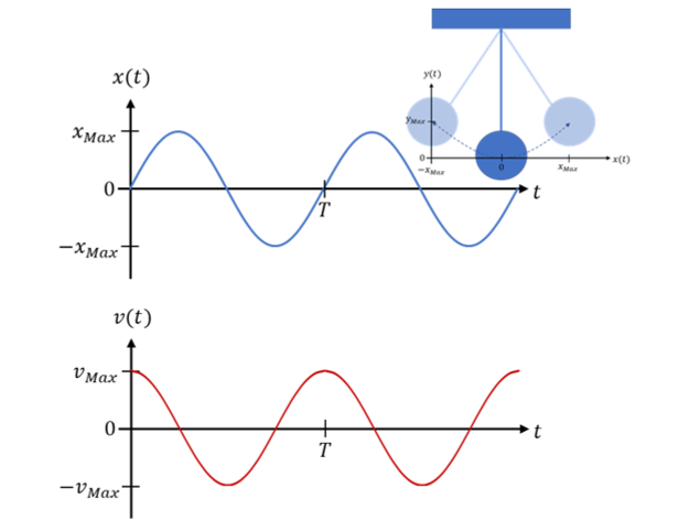
Time curves of the position x(t) and the speed v(t) of the pendulum

\[ v_x(t) = \frac{dx(t)}{dt} = \frac{d}{dt}\bigl(x_{\mathrm{max}} \cdot \sin(\omega t)\bigr) = x_{\mathrm{max}} \cdot \omega \cdot \cos(\omega t) = v_{\mathrm{max}} \cdot \cos(\omega t) \]

For the kinetic energy we need the square of the speed, v².

\[ \begin{gathered} v_x^2(t) = v_{\mathrm{max}}^2 \cdot \cos^2(\omega t) = \frac{v_{\mathrm{max}}^2}{2} \bigl(1 + \cos(2\omega t)\bigr) \\[6pt] W_{\mathrm{Kin}} = \frac{1}{2} m \cdot v^2 = \frac{1}{2} m \cdot \frac{v_{\mathrm{max}}^2}{2} \bigl(1 + \cos(2\omega t)\bigr) \\[6pt] \text{With } W_{\mathrm{Kin,max}} = \frac{1}{2} m \cdot v_{\mathrm{max}}^2 \\[6pt] W_{\mathrm{Kin}} = \frac{W_{\mathrm{Kin,max}}}{2} \cdot \bigl(1 + \cos(2\omega t)\bigr) \\[6pt] \Delta W_{\mathrm{Pot}} = \frac{W_{\mathrm{Pot,max}}}{2} \cdot \bigl(1 - \cos(2\omega t)\bigr) \end{gathered} \]

The two forms of energy have very similar shapes. The peak values are equal, because the energy is converted completely from kinetic energy into potential energy (and vice versa). We can now draw the basic curves of the two forms of energy involved:

\[ \begin{gathered} W_{\mathrm{Kin,max}} = W_{\mathrm{Pot,max}} = W_{\mathrm{Max}} \\[6pt] W_{\mathrm{Kin}} = \frac{W_{\mathrm{Max}}}{2} \cdot \bigl(1 + \cos(2\omega t)\bigr) \\[6pt] \Delta W_{\mathrm{Pot}} = \frac{W_{\mathrm{Max}}}{2} \cdot \bigl(1 - \cos(2\omega t)\bigr) \\[6pt] \Delta W_{\mathrm{Pot}} + W_{\mathrm{Kin}} = W_{\mathrm{Max}} \end{gathered} \]

The sum of the two energies in the system is the same at every moment. The energy does not decrease or increase; it only alternates between the two forms of energy.

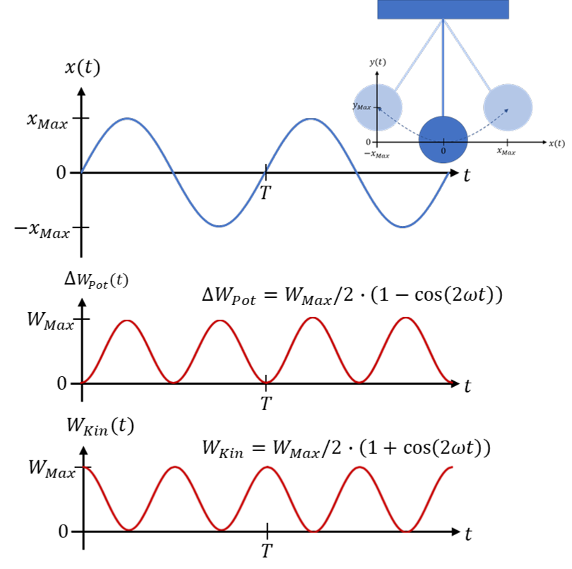
Time curves of the position x(t), the potential energy ΔW_Pot(t) and the kinetic energy W_Kin(t) of the pendulum

At the point of lowest potential energy (dark blue starting position of the pendulum), the kinetic energy is at its maximum. Here the pendulum swings past quickly. In an end position of the oscillation (light blue pendulum position), there is no speed and therefore no kinetic energy. Instead, the potential energy is at its maximum. Between the extreme values, the energies change sinusoidally with a 180° phase shift relative to each other.

All other examples of oscillations with two forms of energy follow similar formulas. The energy is shifted sinusoidally back and forth between the two forms of energy involved. The total energy in the system remains constant.