Electrical Engineering BMT & UFC › Energy Storage › Water Reservoir

Graphical Solution

A graphical approach lends itself to these relationships: the integral of the time curve of a quantity equals the area under the time curve. The example is extended so that the fill level does not change at all for 10 seconds, is then filled for 10 seconds and, after filling, is emptied for 20 seconds.

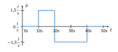
Inflow v̇ over time: 10 s no change, 10 s filling, 20 s emptying

\[ \begin{gathered} \text{Initial value } h_0(t_{\mathrm{Start}}) = 15\,\mathrm{cm} \\[4pt] \text{no change for } 10\,\mathrm{s} \\[4pt] \text{filling for } 10\,\mathrm{s} \text{ with } \dot{v} = 1.5\,\frac{\mathrm{l}}{\mathrm{s}} \\[4pt] \text{emptying for } 20\,\mathrm{s} \text{ with } \dot{v} = -1.5\,\frac{\mathrm{l}}{\mathrm{s}} \end{gathered} \]

During the first 10 seconds, the fill level does not change. During this time, we evidently do not need any calculation to establish that the fill level is still h = 15 cm at the time t = 10 s.

For the graphical solution of the integrals, the areas under the graph of the filling over time are determined. The following applies: the integral equals the area under the curve that is integrated.

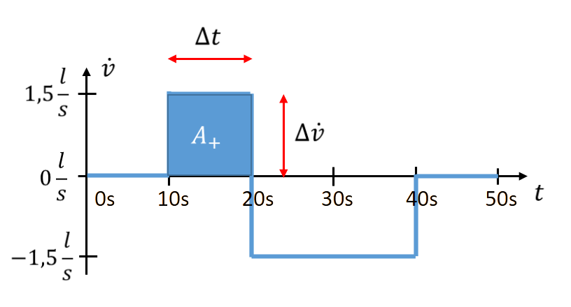
\[ \begin{gathered} \int_{10\,\mathrm{s}}^{20\,\mathrm{s}} \dot{v}(t)\,dt = A_+ \\[4pt] A_+\text{: marked area from the graph} \\[4pt] A_+ = \Delta\dot{v} \cdot \Delta t = 1.5\,\frac{\mathrm{l}}{\mathrm{s}} \cdot 10\,\mathrm{s} = 15\,\mathrm{l} = 0.015\,\mathrm{m}^3 \end{gathered} \]

Area A+ under the inflow between 10 s and 20 s

After 10 seconds, the filling takes place. In the formula, the integral is replaced by the area. The following applies:

\[ \begin{gathered} h(20\,\mathrm{s}) = \frac{1}{A} \cdot \int_{10\,\mathrm{s}}^{20\,\mathrm{s}} \dot{v}(t)\,dt + h_0(10\,\mathrm{s}) = \frac{1}{A} \cdot A_+ + h_0(10\,\mathrm{s}) = \frac{1}{0.1\,\mathrm{m}^2} \cdot 0.015\,\mathrm{m}^3 + 0.15\,\mathrm{m} = 0.3\,\mathrm{m} \\[6pt] \text{with } \int_{10\,\mathrm{s}}^{20\,\mathrm{s}} \dot{v}(t)\,dt = A_+ = 0.015\,\mathrm{m}^3 \end{gathered} \]

The area under the curve of the filling process generally does not have the unit square metre. It is a calculation trick to simplify integral calculus. For this, you have to ignore the units. The unit of this “area” is the product of the units on both axes (here l/s and s).

The result obtained by calculating the area equals the one obtained with the antiderivative. This shows by way of example that the area method is permissible. Areas are often easier to determine than antiderivatives. Of course, these areas are not always rectangles. You can also use the area to determine integrals of very complex functions. The method is particularly advantageous for real measured curves when you need an estimate of the integral over the curve.

Let us apply the method to the emptying process:

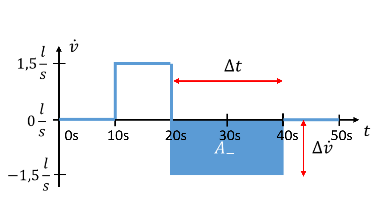
\[ \begin{gathered} \text{Initial value: } h_0(20\,\mathrm{s}) = 30\,\mathrm{cm} \\[4pt] \dot{v} = -1.5\,\frac{\mathrm{l}}{\mathrm{s}} \\[4pt] t_{\mathrm{Start}} = 20\,\mathrm{s} \\[4pt] t_{\mathrm{Ende}} = 40\,\mathrm{s} \\[6pt] h(40\,\mathrm{s}) = \frac{1}{A} \int_{t_{\mathrm{Start}}}^{t_{\mathrm{Ende}}} \dot{v}(t)\,dt + h_0 = \frac{1}{A} \int_{20\,\mathrm{s}}^{40\,\mathrm{s}} (-1.5)\,\frac{\mathrm{l}}{\mathrm{s}} \cdot dt + 30\,\mathrm{cm} \\[6pt] \text{Area } A_- = \Delta\dot{v} \cdot \Delta t = -1.5\,\frac{\mathrm{l}}{\mathrm{s}} \cdot 20\,\mathrm{s} = -30\,\mathrm{l} = -0.03\,\mathrm{m}^3 \end{gathered} \]

Area A− under the inflow between 20 s and 40 s

So for the fill level at the time t = 40 s, the following applies:

\[ \begin{gathered} h(40\,\mathrm{s}) = \frac{1}{A} \cdot \int_{20\,\mathrm{s}}^{40\,\mathrm{s}} \dot{v}(t)\,dt + h_0(20\,\mathrm{s}) = \frac{1}{A} \cdot A_- + h_0(20\,\mathrm{s}) = \frac{1}{0.1\,\mathrm{m}^2} \cdot (-0.03\,\mathrm{m}^3) + 0.3\,\mathrm{m} = 0\,\mathrm{m} \\[6pt] \text{with } \int_{20\,\mathrm{s}}^{40\,\mathrm{s}} \dot{v}(t)\,dt = A_- = -0.03\,\mathrm{m}^3 \end{gathered} \]

At the end, the bucket is empty. When looking at the emptying of the bucket, the graph immediately shows that the area below the time axis is twice as large as the area above the time axis. Twice as much water is drained from the bucket as was filled into it before.

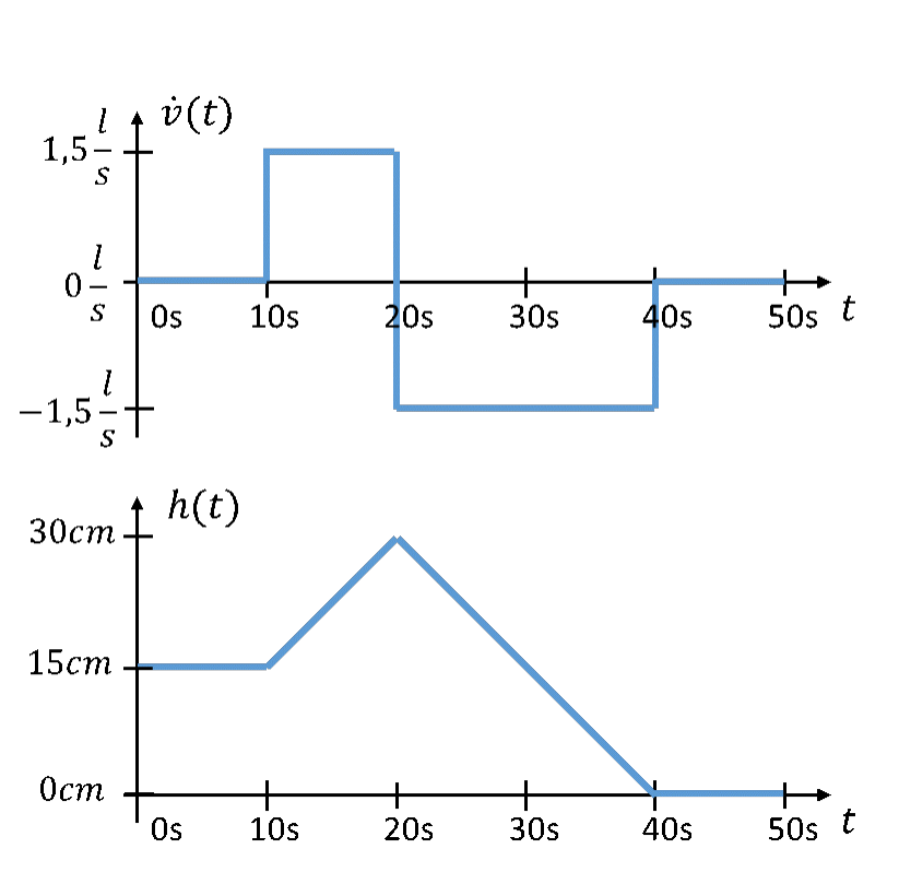
During the periods in which there is neither inflow nor outflow, the fill level does not change.

So far, we have calculated the fill level at fixed points in time. With constant filling, the curve between these points in time is linear.

Inflow v̇(t) and fill level h(t) over time

The intuitive example of the bucket is used in the following chapter to explain the behaviour of electrical energy stores.