Measurement Technology › Filters Part 1 › Electrical Filters

Filter Design

The filter is characterised by its cut-off frequency. So far we have assumed it to be a fixed value and checked how signals are changed by the filter. In practice, the procedure is exactly the other way round. You have signals and want to influence them with a particular filter.

The useful signal should pass the filter unchanged. We want to reduce the peak value of the interference signals as much as possible. Let us build a suitable filter for this. How must the cut-off frequency of the filter be chosen so that both conditions are optimally fulfilled? To answer this, we first look at an example and derive the general procedure from it.

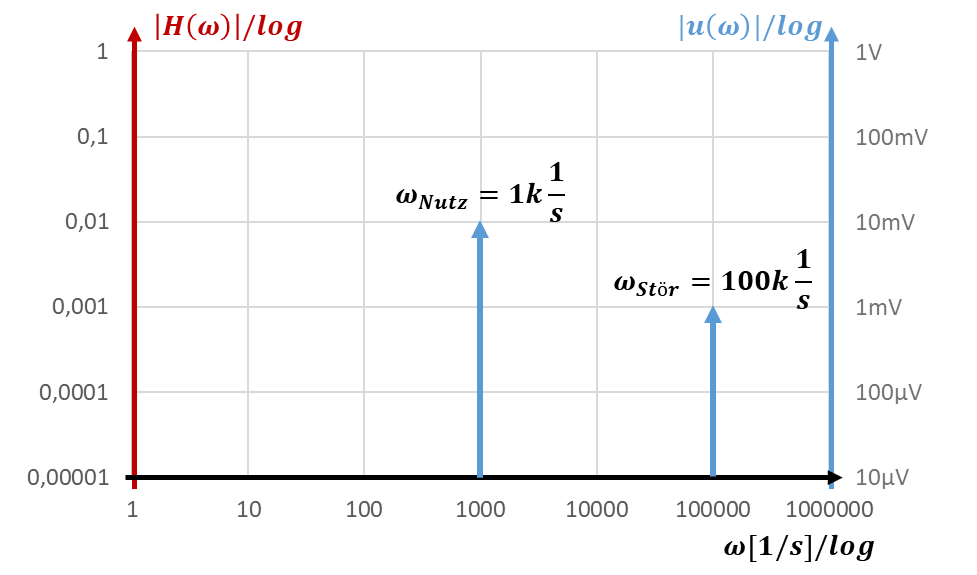
Spectrum with useful signal at ω_Nutz = 1k 1/s and interference signal at ω_Stör = 100k 1/s — Nutz = useful

In the Bode plot above you see on the left a y-axis for the transfer function |H(ω)| in red. On the right you see a further y-axis in blue for voltages. In one diagram we show peak values of signal voltages (blue) and a filter transfer function (red). In the first step we look only at the voltages. A useful signal with a peak value of 10 mV and angular frequency ω_Nutz = 1k 1/s is shown by the middle arrow. An interference signal with a peak value of 1 mV and angular frequency ω_Stör = 100k 1/s is shown by the right arrow (Nutz = useful, Stör = interference).

The signals are actually points, not arrows. The tips of the arrows point to the points that represent the peak values of the voltages on the right-hand axis.

Next we place a transfer function |H(ω)| in red in the diagram so that the filter lets the useful signal pass unchanged with |H(ω_Nutz)| = 1. Because the filter already has a gain of |H| ≈ 0.7 at the corner frequency, we always place the cut-off frequency of the filter at least a factor of 10 higher than the useful frequency.

\[ \omega_g \ge 10 \cdot \omega_{\mathrm{Nutz}} \]

Let us first set the cut-off frequency to ω_g = 10k 1/s. The corresponding Bode plot looks like this:

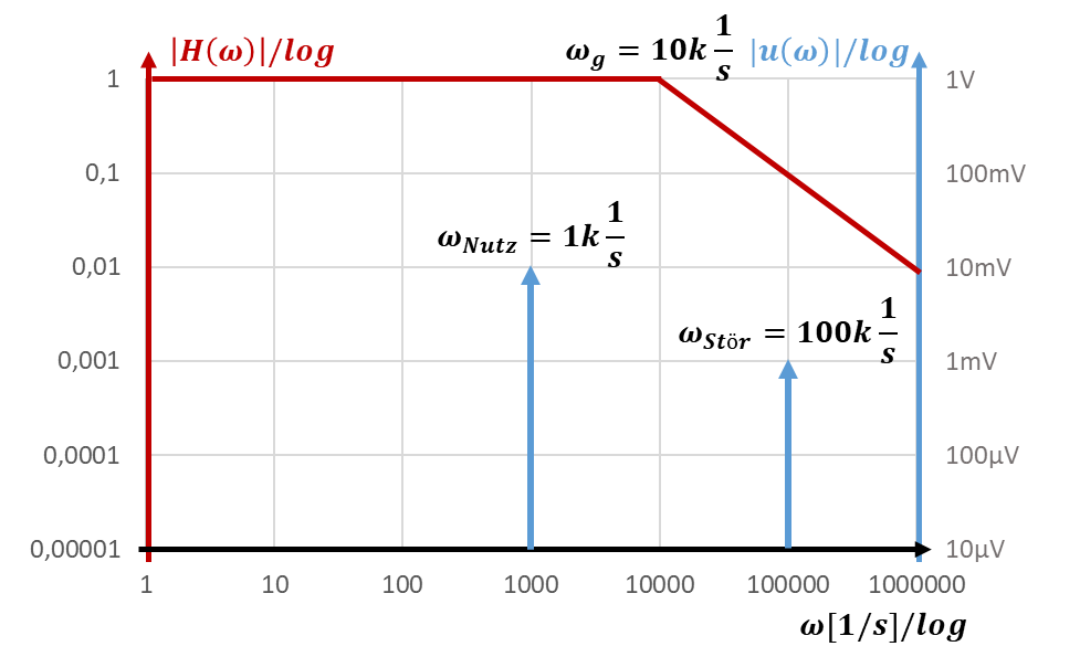
Low-pass filter with ω_g = 10k 1/s: useful signal unchanged, interference signal attenuated — Nutz = useful

The filter with the red Bode plot amplifies the useful signal with |H(ω_Nutz)| = 1 and the interference signal with |H(ω_Stör)| = 0.1. You can read this gain from the y-value of the left-hand axis at the respective signal frequencies.

Another filter with the cut-off frequency ω_g = 100k 1/s looks like this:

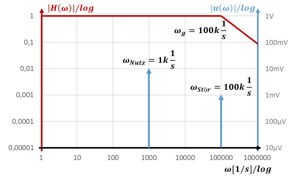
Low-pass filter with ω_g = 100k 1/s: interference signal hardly attenuated — Nutz = useful

This filter also amplifies the interference signal with |H(ω_Stör)| = 1 (with Bode approximation) or, more precisely, with |H| ≈ 0.7 (without Bode approximation). The peak value of the interference signal is hardly reduced by this filter. The filter with the cut-off frequency at ω_g = 10k 1/s is more suitable. In general:

A filter works better the further its cut-off frequency is from an interference frequency.

Calculating the gain

You use the Bode plot as a simplification so that you no longer have to calculate. You can still calculate the gain of a filter, though. To do so, insert into the transfer function the angular frequency ω at which you want to calculate the gain. We use a new example:

\[ \begin{gathered} \omega_g = 10\mathrm{k}\,\tfrac{1}{\mathrm{s}},\quad \omega_{\mathrm{Nutz}} = 1\mathrm{k}\,\tfrac{1}{\mathrm{s}},\quad \omega_{\mathrm{Stör},1} = 100\mathrm{k}\,\tfrac{1}{\mathrm{s}},\quad \omega_{\mathrm{Stör},2} = 1\mathrm{M}\,\tfrac{1}{\mathrm{s}} \\[6pt] |H(\omega)| = \frac{1}{\sqrt{1 + (\omega/\omega_g)^2}} \\[6pt] |H(\omega_{\mathrm{Nutz}})| = \frac{1}{\sqrt{1 + \left(1\mathrm{k}\,\frac{1}{\mathrm{s}} / 10\mathrm{k}\,\frac{1}{\mathrm{s}}\right)^2}} = \frac{1}{\sqrt{1 + (0.1)^2}} = \frac{1}{\sqrt{1.01}} \approx 1 \\[6pt] |H(\omega_{\mathrm{Stör},1})| = \frac{1}{\sqrt{1 + \left(100\mathrm{k}\,\frac{1}{\mathrm{s}} / 10\mathrm{k}\,\frac{1}{\mathrm{s}}\right)^2}} = \frac{1}{\sqrt{1 + 10^2}} = \frac{1}{\sqrt{101}} \approx \frac{1}{10} = 0.1 \\[6pt] |H(\omega_{\mathrm{Stör},2})| = \frac{1}{\sqrt{1 + \left(1\mathrm{M}\,\frac{1}{\mathrm{s}} / 10\mathrm{k}\,\frac{1}{\mathrm{s}}\right)^2}} = \frac{1}{\sqrt{1 + 100^2}} \approx \frac{1}{100} = 0.01 \end{gathered} \]

Attenuation

The attenuation is the reciprocal of the gain. The term has become established in measurement technology, although all effects can already be described with the gain. If a signal is amplified by a factor of 0.01, for example, we can also say that it is attenuated by a factor of 100. It is linguistically more catchy to say that a signal is attenuated by a factor of 100 than that it is amplified by 0.01. As a formula (D = Dämpfung, attenuation):

\[ D(\omega) = \frac{1}{|H(\omega)|} \]

The attenuation – just like the gain – depends on the frequency. Attenuation is only a new word without any real new meaning.

Frequency and angular frequency

So far, all calculations have been carried out with the angular frequency ω. The angular frequency is not a very intuitive quantity. You can also carry out all filter considerations with the frequency f. The following applies:

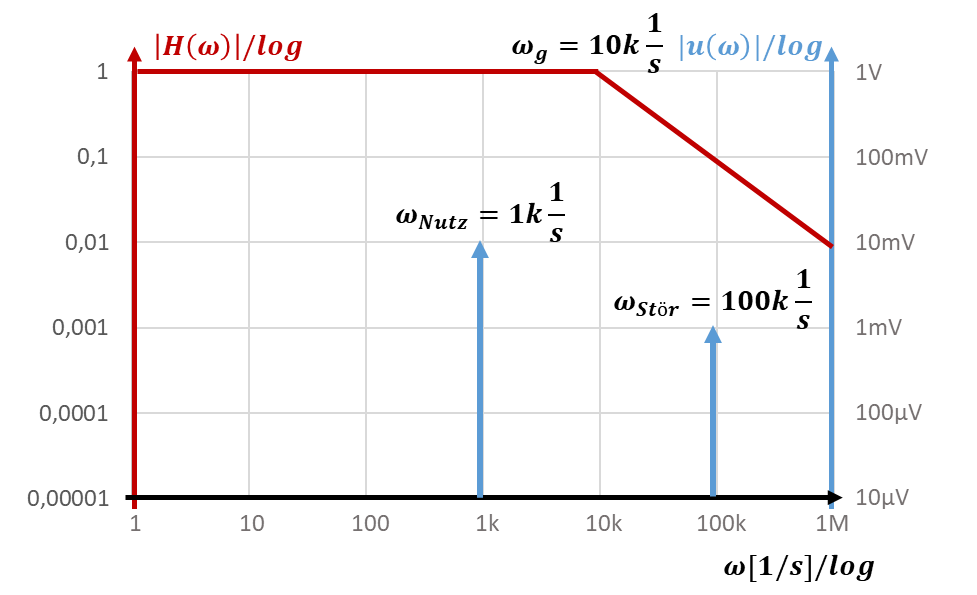
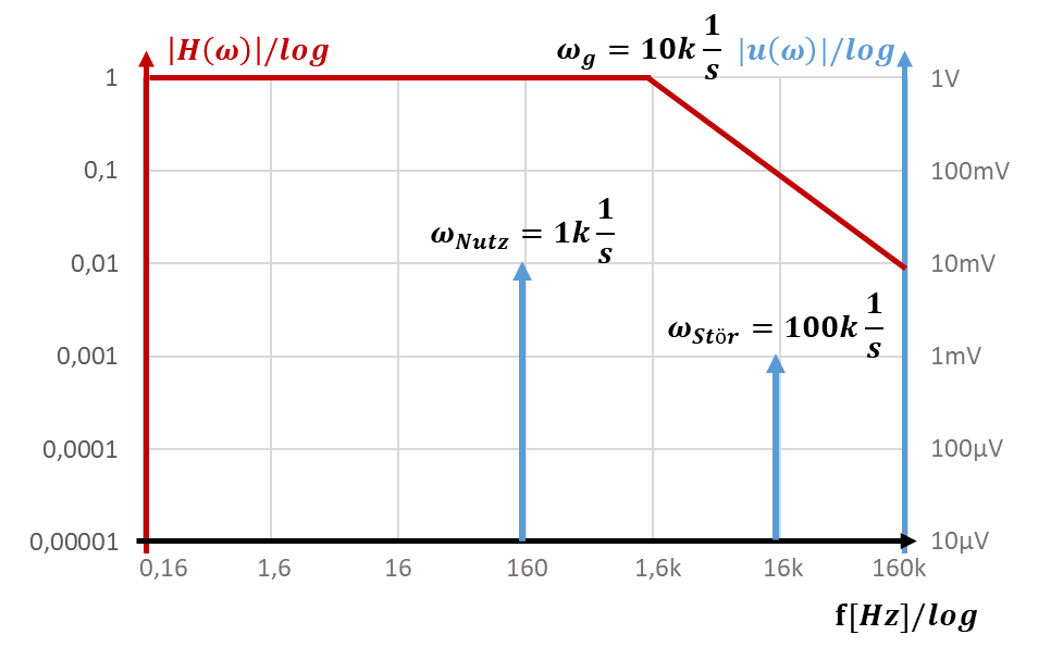
\[ \begin{gathered} \omega = 2\pi \cdot f \\[6pt] f = \frac{\omega}{2\pi} \\[6pt] \omega_g = \frac{1}{RC},\quad f_g = \frac{1}{2\pi RC} \end{gathered} \]

In practice you will encounter both representations. If you choose the form with ω, calculating the cut-off frequency is easier, because the factor 2π is omitted. Frequencies are usually given as f. At the power socket, for example, f = 50 Hz is present. You can convert this frequency into an angular frequency of ω = 314 1/s. In the Bode plot, the values on the x-axis change by the factor 2π if you plot it over f. This is shown by the following Bode plot with the angular frequency ω and then with the frequency f on the x-axis. Look at the x-axes of the two following figures to see the difference.

Bode plot over the angular frequency ω with axis labels 1k, 10k, 100k, 1M — Nutz = useful

The same Bode plot over the frequency f in Hz (0.16 Hz to 160 kHz) — Nutz = useful