Systematic Measurement Errors

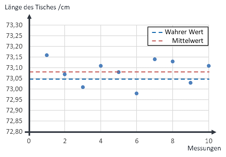
Systematic measurement deviations all point in the same direction. We carry out 10 successive measurements of the length of the same table with a folding rule that is 0.8 mm too short. We then obtain 10 measured values whose mean is a result corrected for chance. But because of the length of the folding rule, all measured values are slightly higher than in the series of measurements with the ideal folding rule in the previous chapter, so the mean lies slightly above the previous mean.

The measured values around 73.05 cm are then not all 0.8 mm too large, but only proportionally by

\[ \Delta l = 0.8\,\mathrm{mm} \cdot \frac{73.05\,\mathrm{cm}}{2\,\mathrm{m}} = 0.3\,\mathrm{mm} \]

too large. A deviation in the length of the folding rule causes a slope error, which enters the measurement result as a factor. The same measurements as in the last example give the following result with the folding rule that is too short:

Measurement	Measured value in cm
1	73.16
2	73.07
3	73.01
4	73.11
5	73.08
6	72.98
7	73.14
8	73.13
9	73.03
10	73.11
Mean	73.08

In the graphical representation, you can recognise the effect of systematic errors as a shift of the mean:

Measured values of the table length with true value 73.05 cm and mean 73.08 cm shifted by the systematic deviation — Länge = length · Tisches = table · Wahrer Wert = true value · Mittelwert = mean value · Messungen = measurements

If we measure a table of twice the length with the same folding rule, the deviation of the mean from the true value is

\[ \Delta l = 0.8\,\mathrm{mm} \cdot \frac{146.10\,\mathrm{cm}}{2\,\mathrm{m}} = 0.6\,\mathrm{mm} \]

So to correct a slope error, we cannot simply subtract a constant value from the result as with an offset error; we need a correction factor. The systematic error can be of any type (offset, slope, linearity etc.). We correct it in each case with the methods you have learned in the previous chapters.

Random deviations between several measurements of the same measurement system can easily be corrected via the mean. The only disadvantage is that you first have to measure many values, then average them and only then output a result. So there is a time delay between the time of measurement and the time of output.

Random deviations between all measurement systems from one production run are more difficult to correct. Because all systems – if we only look closely enough, down to the last decimal place – determine different measured values for the same measurement, the random measurement deviations must be determined individually for each device. If it turns out, for example, that all measuring instruments measure wrongly by the same value, it is a systematic error.

The effort required to correct systematic errors is relatively low. The error is determined once and then corrected in the same way in every system in the digital signal processing. Random errors must be determined and corrected individually in each system with great effort. The correction effort in digital signal processing is always high when, for example, the inverse function of an unknown non-linear characteristic that differs in each system has to be found. This effort is necessary to build high-precision measurement systems. It justifies part of the high prices of high-quality measurement technology.

Summary

For normally distributed quantities, we use the following formulas:

\[ \begin{gathered} \text{True value } x_{\mathrm{wahr}} \\[6pt] \text{Mean } \bar{x} = \frac{1}{N} \sum_{n=1}^{N} x_n \\[6pt] \text{Systematic deviation of the mean from the true value: } x_{\mathrm{sys}} = \bar{x} - x_{\mathrm{wahr}} \\[6pt] \text{Random deviation of a quantity } x \text{ from the mean: } x_{\mathrm{stoch}} = x - \bar{x} \end{gathered} \]