At the end of the last chapter we already changed the transient behaviour of PT1 behaviour with a controller parameter. The transient behaviour of PT1 behaviour is described by the parameter τ. τFÜ depends on kIR when we control a P system with an I controller.
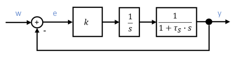
Now let us look at a second-order system in an example. The system consists of I behaviour and PT1 behaviour. Because of the I behaviour in the system, the controlled system has no steady-state control error. We can optimise the transient behaviour with a P controller. The control loop looks like this:
First we simplify the loop for the calculation. It contains three terms describing the gain. We can combine them into one term.
After this transformation, the result resembles the standard form of oscillating PT2 behaviour. Now we can determine the characteristic parameters by comparing coefficients:
\[
\begin{gathered}
H_{\mathrm{FÜ}} = H_{\mathrm{PT2}} = \frac{1}{\frac{\tau_S}{k} \cdot s^2 + \frac{1}{k} \cdot s + 1} = \frac{k_{P,\mathrm{PT2}}}{\frac{1}{\omega_0^2} s^2 + \frac{2D}{\omega_0} s + 1} \\[8pt]
\text{Numerator: } k_{P,\mathrm{PT2}} = 1 \\[8pt]
\text{Denominator, coefficient of } s^2\text{: } \frac{1}{\omega_0^2} = \frac{\tau_S}{k} \rightarrow \omega_0 = \sqrt{\frac{k}{\tau_S}} \\[8pt]
\text{Effect of } k_{PR} \text{ on the oscillation frequency: } \omega_0 \sim \sqrt{k_{PR}} \\[8pt]
\text{Denominator, coefficient of } s\text{: } \frac{2D}{\omega_0} = \frac{1}{k} \rightarrow D = \frac{\omega_0}{2k} = \frac{1}{2} \sqrt{\frac{1}{k \cdot \tau_S}} \\[8pt]
\text{Effect of } k_{PR} \text{ on the damping: } D \sim \sqrt{\frac{1}{k_{PR}}}
\end{gathered}
\]
We can influence parameter k directly via the controller’s kPR. Parameter k acts on the oscillation frequency and the damping of the controlled system. So the controller settings influence the transient behaviour of the controlled system.