Water Model
The chapter “Water model” is not relevant for the exam. I hope it helps your understanding. If you only want to prepare quickly for the lecture, skip this chapter.
Filtering effect of a radiator
There is a good everyday example that illustrates the effect of a filter. We look at an ordinary radiator with a rotary valve that you can open and close by hand. When you open it, the radiator gets warm. The input of the system is the valve. The output is the temperature of the radiator.
If you open the radiator fully and then close it fully again once every second, how does its temperature change? Not at all. Such fast changes at 1 Hz at the valve do not cause the radiator to change its temperature just as quickly. If you open the same valve fully every half hour and close it again after another half hour, the temperature of the radiator does change. It becomes alternately warm and cold.
A fast change in the input quantity (valve position) does not lead to a change in the output quantity (temperature). Fast or high-frequency signals at the input are not visible at the output. A slow or low-frequency change at the input every half hour is visible at the output. So a radiator forms a filter, because it transfers changes in the input quantity to the output quantity to different degrees depending on the signal frequency.
The rest of this chapter is not relevant for the exam. It attempts to explain the effect of filters intuitively using the water model. If you only want to prepare for the lecture with little effort, simply leave out the entire rest of “Understanding filters”.
Water model of the filter
Many electrical relationships between voltage and current can be visualised with the water model. However, some students find the explanation of filters using the water model not very helpful. If you notice that the water model does not help your understanding, simply skip this chapter.
For an intuitive explanation of how filters work, we look at the water model from Fundamentals of Electrical Engineering. If you took that course a long time ago, take the time to read the chapter again. We show the effect of filters with the water model. Afterwards you will also understand it for electrical filters.
Let us look at AC signals in the water model. To model sensors, we need AC voltage sources. We need a water source whose output value changes sinusoidally. In the water model, this is a huge lake whose height changes sinusoidally. We do not consider negative voltages, i.e. no negative heights in the water model. That would be too complicated. A source whose height changes over time can be visualised as follows:
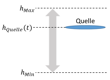
To avoid negative heights, we set hMin = 0 m. The height of water is analogous to voltage in electrical engineering. The higher the lake is drawn, the higher the voltage of the electrical voltage source that the lake represents. An electrical filter can also have negative voltages applied.
Filters always consist of a combination of limiting elements such as resistors and storage elements in one circuit section. In the water model, a pipe stands for an ohmic resistor. The resistance increases as the diameter of the pipe decreases. The slope of the pipe stands for the voltage across the resistor. The water flow (current) through the pipe is determined by its slope and its diameter.
The bucket is the storage element in the water model. For a bucket, the fill level is the voltage and the inflow/outflow is the current.
Modelling a filter
A pipe is installed between a source and a bucket. The height of the source is variable. The height of the bucket is not, but the fill level of the bucket can change its height. One end of the pipe is attached to the source. When the source changes its height, this end of the pipe moves up and down with it. The other end of the pipe is attached to the bucket. It floats on the water and always changes its height with the fill level of the bucket. So both ends of the pipe can change their height.
The following figures show several combinations of bucket fill level and source height. What matters in each case is the direction in which the water flows and how large the height difference across the pipe is. From this we determine the inflow and outflow rate of the bucket.
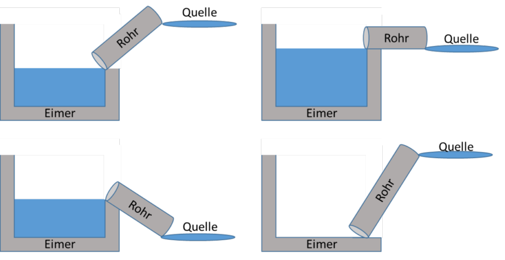
In the top left figure, the half-filled bucket is filled from a source whose height is above the bucket’s fill level. More water flows from the source into the bucket. In the bottom left figure, the bucket is also half full. The height of the source is below the bucket’s fill level. Water flows from the bucket into the source. The top right figure shows a case where the bucket’s fill level and the source are at the same height. No water flows. This state can be reached at any height.
The inflow of water from the source into the bucket (or vice versa) is limited in this system. It is at its maximum in the bottom right figure and directed towards the bucket. For this, the source must be at its maximum height and the bucket must be completely empty. No more water can flow through the pipe than in this case. The rate of inflow and outflow determines how quickly the fill level of the bucket changes. It is set by the slope and the diameter of the pipe.
The right wall of the bucket is in the way in the drawings. It simply always moves so that water can flow. When the fill level of the bucket falls, the wall moves down a little further so that the level can keep falling. So this wall is never in the way. The water analogy is not perfect for filters; unfortunately it needs this unattractive workaround.
To generate an AC signal, the source is now moved up and down sinusoidally. As a result, the intensity and direction of the water flow into the bucket change constantly. This constantly changes the fill level of the bucket.
The fill level of the bucket follows the height of the source. The two are coupled via the pipe. Source, pipe and bucket form a series circuit.
Influencing the filter
We can influence the peak value of the bucket’s fill level via three parameters. In our minds we always change one of the parameters and keep the other two unchanged.
1. Pipe diameter: if we fill a bucket through a drinking straw with a very small diameter, it takes a long time. The fill level of the bucket changes more slowly than with a pipe of large diameter.
2. Base area of the bucket: if we fill a swimming pool instead of the bucket, the fill level changes less. Again, the fill level changes more slowly for a bucket with a larger base area.
3. Frequency: if we change the height of the source faster, we increase the frequency of the signal at the source. There is then less time available to fill and empty the bucket. Less water is moved through the pipe per sine half-wave than with a slow movement. This is due to the limitation of the maximum water flow by the pipe diameter.
If the pipe is thin and the base area of the bucket is large, the fill level of the bucket can no longer keep up at a high sine frequency. The bucket is no longer completely emptied and filled. The fill level of the bucket lags behind the height of the source in time. This effect is exploited in filtering. It is what this chapter is about.
We start with a low frequency, a large pipe diameter and a small bucket area. So we fill a tiny thimble very slowly through a really large sewer pipe. The maximum possible water flow is much larger than the water flow needed to keep the bucket’s fill level at source height at all times. The fill level of the bucket therefore changes almost without delay as soon as the height of the source changes.
The peak value of the source movement is chosen so that the bucket is always completely filled and completely emptied. The source height “Max” is therefore high enough for the bucket to be completely filled. The source height “Min” corresponds to the height of the bucket’s bottom. A time curve of filling and emptying looks like this:
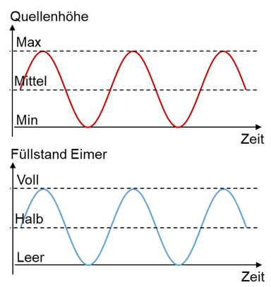
Now we take a thinner straw as the pipe and a much larger bucket, and we move the source up and down faster. The maximum possible water flow is now smaller than the water flow that would be needed to keep the bucket’s fill level at source height at all times. The fill level of the bucket therefore no longer reaches the peak values full and empty. It follows the height of the source with a time delay. A time curve then looks roughly like this:
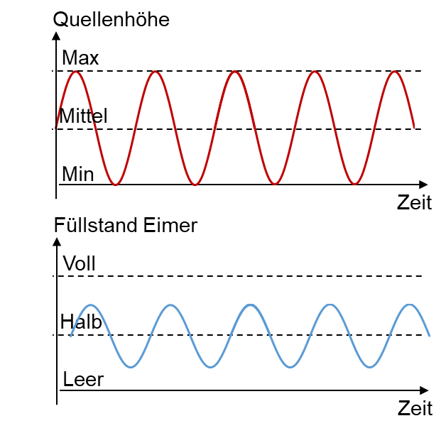
We obtain a phase shift between source height and bucket fill level. The peak value of the bucket’s fill level is lower than that of the source height. To intensify this effect further, we reduce the cross-sectional area of the pipe, increase the area of the bucket or increase the frequency of the source’s sine.
The faster the height of the source changes, the less the fill level of the bucket changes. With this we have already built a filter. The input quantity of the filter is the source height. The output quantity is the fill level of the bucket. The filter acts differently on signals depending on their frequency. The higher the frequency of the signals at the input, the lower the peak value of the signals at the output of the filter.
Useful signal and interference signal
Imagine that the source contains two signals: a low-frequency useful signal and a high-frequency interference signal. The source moves slowly up and down with the useful signal. It has the frequency fNutz and the peak value hNutz. This movement is superimposed by a fast movement with the frequency fStör and the peak value hStör of the interference signal. We need the constant height hMittel in the formula so that the height moves as an AC signal around the mean height (Nutz = useful, Stör = interference, Mittel = mean).
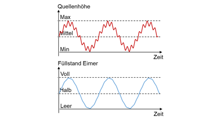
The fill level of the bucket follows the slow useful signal completely. Because the source height changes slowly, a lot of water is moved. The pipe is thick enough to change the bucket’s fill level with this water, because the bucket’s area is small relative to the amount of water moved.
The fast interference signal has to pass through the same pipe and fill the same bucket. At the high frequency, however, much less water is moved. The pipe is too thin to change the fill level noticeably with the small amount of water, given the large area of the bucket. Therefore the interference signal is less visible in the bucket’s fill level than in the source height.
Via the pipe diameter and the bucket area, we can influence up to which frequency signals from the source should still be fully visible in the bucket’s fill level. So if we know the frequencies of the interference signal and the useful signal, we can adapt the bucket and pipe accordingly. This is how filters are built. Once the filter has been built, the pipe diameter and bucket area are fixed parameters. Only the frequency at which the source height changes then varies with the applied signals.
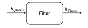
Let us look at a block diagram of the set-up. The source height is the input quantity. The fill level of the bucket is the output quantity. We define a transfer function for the filter. It contains the mathematics of filters, which we will look at next (Quelle = source, Eimer = bucket).