Control Engineering › Oscillating Systems 1

Oscillating Control Loops

We now leave the pendulum behind and look at a general controlled system. Systems capable of oscillation oscillate by themselves when excited, without much having to happen from outside. Controllers ensure that the controlled variable matches the reference variable. What happens if a system capable of oscillation is integrated into a control loop and the reference variable is constant? The controller then tries to keep the controlled variable constant. The system tends to oscillate at the slightest excitation, which results in a non-constant controlled variable. Who wins, the controller or the tendency to oscillate?

A system capable of oscillation knows two stable states. It can be kept at rest and simply not “move”. Or it oscillates sinusoidally. In an oscillation, we can influence how the peak value changes over time.

A “good” control loop with a constant reference variable always tries to reach the state of rest. To do this, it reduces the peak value of the oscillation through damping. When the controller excites the system, it usually starts to oscillate at first. It is one of the most difficult tasks in control engineering to design a controller so that this oscillation is damped and the controlled variable becomes constant in the shortest possible time.

When the reference variable performs a setpoint step, e.g. a heating system is to raise the room temperature from 20 °C to 25 °C, the actuator reacts by driving the plant differently. For a system capable of oscillation, this acts like pushing a pendulum. It is set into oscillation. To analyse the problem, we break it down into parts and put it back together at the end. First, let us look at part of the control loop in isolation: an actuator drives a plant in a system capable of oscillation.

Actuator and plant

The pendulum example in the control loop is too complicated to consider further here. So we leave the pendulum example and look in general at an actuator with P behaviour that drives a plant with P behaviour. Suppose the controlled variable is already oscillating in a damped manner. So the peak value of the oscillation decreases over time. Via the actuator, we can either damp the oscillation further or maintain or amplify it.

To maintain the oscillation, the actuator must act in phase with the controlled variable. The phase shift between actuator and plant must be 0. Then the actuator always acts so that the controlled variable is “supported”.

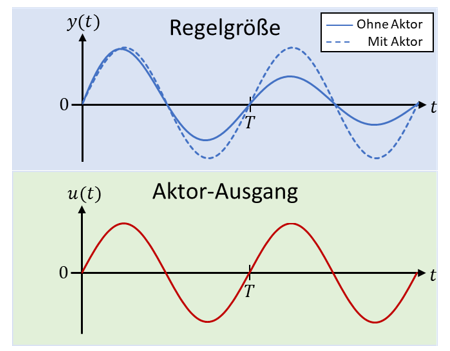
Positive feedback: controlled variable y(t) without and with actuator, and actuator output u(t) in phase — Regelgröße = controlled variable · Aktor-Ausgang = actuator output · Aktor = actuator

\[ \text{Positive feedback: actuator supports the controlled variable} \]

The actuator output (red) is a quantity that acts on the controlled variable (blue) via the plant. Without the actuator, the peak value of the controlled variable would decrease over time because of damping (solid line). Because the actuator always intervenes in the direction of the controlled variable, it counteracts the damping (dashed line). In the special case shown, the energy the actuator adds to the plant exactly equals the energy that damping withdraws from it. That is why the peak value of the oscillation remains constant. If the energy supplied exceeds the damping, the peak value increases over time. We speak of “positive feedback” when the actuator supports or amplifies the controlled variable.

Conversely, if an oscillation is to be damped by the actuator, the actuator must act 180° out of phase with the controlled variable. Then the actuator always pulls the controlled variable in the direction opposite to its current movement.

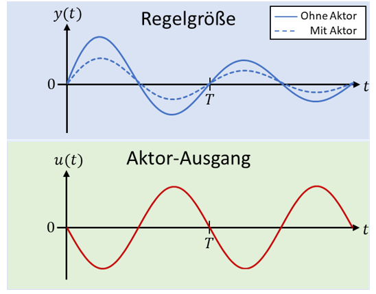
Negative feedback: controlled variable y(t) without and with actuator, and actuator output u(t) in antiphase — Regelgröße = controlled variable · Aktor-Ausgang = actuator output · Aktor = actuator

\[ \text{Negative feedback: actuator counteracts the controlled variable} \]

Note the phase shift between actuator and controlled variable. The actuator acts against the “direction” of the controlled variable. With negative feedback, the actuator acts as additional damping. The peak value of the oscillation decreases faster as a result of the intervention.

Opened control loop

The analysis of systems capable of oscillation must include the entire control loop. For this, the closed control loop is opened at any point. We usually open it between the output of the plant and the controlled variable. This gives us a form of calculation from which we can directly infer how the control changes the oscillation:

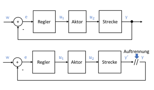
Control loop of controller, actuator and plant, below it with the feedback opened between y′ and y — Regler = controller · Aktor = actuator · Strecke = plant · Auftrennung = cut

The upper figure shows the closed control loop, which is opened in the lower figure. To the left of the opening, the quantity y′ comes out of the plant. The quantity y is fed back to the input. Why do we do this? We can now calculate how the quantity y changes when it passes once through the control loop and comes out again as y′. Because we are only interested in the effect of the control loop, we set the reference variable to 0 to reduce complexity.

In practice, no control loop is opened or interrupted; otherwise the control would no longer work. Opening the control loop is only a mathematical trick that helps understanding. The following applies:

\[ \begin{gathered} \text{Simplification: } w = 0 \\[6pt] e = w - y = -y \\[6pt] y' = H_R \cdot H_A \cdot H_S \cdot e = -H_R \cdot H_A \cdot H_S \cdot y \\[6pt] \text{Loop gain: } v_R = \frac{y'}{y} = -H_R \cdot H_A \cdot H_S \end{gathered} \]

We recognise the change of the signal y by the control loop from the quotient y′ divided by y. In the opened control loop, this quotient is called the “loop gain”. All function blocks contribute to the loop gain. If the transfer function of a function block is less than 1, it attenuates the signal. If it is greater than 1, it amplifies the signal. The same applies to the loop gain as the product of all function blocks (including the minus sign at the subtraction point).

Magnitude of the loop gain

If the loop gain is 1, the signal does not change when passing through the control loop. Then y′ = y. Attenuation and amplification cancel each other out. If the magnitude of the loop gain is greater than 1, the signal is amplified overall and y′ > y. The peak value of an oscillation then becomes a little larger with each pass through the control loop. If the magnitude of the loop gain is less than 1, the peak value of an oscillation decreases, because the signal is attenuated overall.

To illustrate this graphically, for different loop gain values I have shown a signal before passing through the control loop in red and after passing through it in blue.

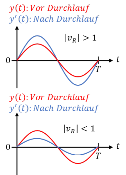
Signal y(t) before and y′(t) after one pass through the control loop for |v_R| > 1 and |v_R| < 1 — Vor Durchlauf = before passing through the loop · Nach Durchlauf = after passing through the loop

If we know how a signal changes in one pass through the control loop, we can determine its time behaviour. If a signal becomes smaller with each pass, it will disappear over time. If it becomes larger with each pass, it will keep growing. The loop gain shows us how a signal will change over time.

Phase of the loop gain

We already know from looking at actuator and plant that it matters at what phase an actuator “pushes” a plant. An actuator can damp or amplify an oscillation, depending on how excitation and oscillation are shifted relative to each other. A 0° shift causes amplification, a 180° shift causes damping. We can transfer these findings to the loop gain:

If a signal undergoes no phase rotation (0°) when passing through the control loop, the signal pushes itself, so that the oscillation is amplified. If the oscillation is currently positive, it becomes even more positive, because after one pass it drives itself with the positive value. The same applies if the phase rotation is n ∙ 360°.

If the phase rotation is 180°, the oscillation damps itself. If the oscillation is currently positive, it becomes negative when passing through the control loop and reduces itself. This applies not only at 180° but also at 180° + n ∙ 360°.

Every control loop contains a subtraction point at its input. It always rotates the phase of the loop gain by 180°. A factor of −1 corresponds to a phase rotation of 180°.

\[ -1 = e^{j\pi} \mathrel{\widehat{=}} e^{j180°} \]

Conditions for oscillation

So an oscillation can only be sustained permanently if two conditions apply:

1. The magnitude of the loop gain equals 1. Then the peak value of the oscillation remains constant. Or it is greater than 1; then the peak value increases.

2. The phase of the loop gain is 0° or n ∙ 360°.

If a control loop is not to oscillate permanently, we must avoid these conditions. We do this by setting either the phase or the magnitude of the loop gain.

Storage elements in the control loop

Every storage element rotates the phase between input and output quantity by 90° or π/2. Integrators and differentiators rotate in opposite directions. For sinusoidal signals:

\[ \begin{gathered} \text{Integrator / I behaviour:} \\[6pt] \text{Output} = \frac{1}{s} \cdot K_I \cdot \text{input} \\[6pt] s = j\omega \\[6pt] \text{Output} = \frac{1}{j\omega} \cdot K_I \cdot \text{input} = \frac{K_I}{\omega} \cdot e^{-j\frac{\pi}{2}} \cdot \text{input} \end{gathered} \]

\[ \begin{gathered} \text{Differentiator / D behaviour:} \\[6pt] \text{Output} = s \cdot K_D \cdot \text{input} \\[6pt] s = j\omega \\[6pt] \text{Output} = j\omega \cdot K_D \cdot \text{input} = \omega \cdot K_D \cdot e^{+j\frac{\pi}{2}} \cdot \text{input} \end{gathered} \]

If two integrators are contained in the control loop, the phase is rotated by 180° overall. Let us look at the loop gain of an opened control loop with an I controller and I behaviour in the actuator:

Opened control loop with controller K_IR = 1, two integrators 1/s, actuator K_IA and plant K_PS — Regler = controller · Aktor = actuator · Auftrennung = cut · Strecke = plant

\[ \begin{gathered} y' = K_{IR} \cdot K_{IA} \cdot K_{PS} \cdot \frac{1}{s^2} \cdot e \\[6pt] e = w - y \text{ with } w = 0 \\[6pt] y' = -K_{IR} \cdot K_{IA} \cdot K_{PS} \cdot \frac{1}{s^2} \cdot y \\[6pt] s = j\omega \\[6pt] y' = +K_{IR} \cdot K_{IA} \cdot K_{PS} \cdot \frac{1}{\omega^2} \cdot y \\[6pt] v_R = \frac{y'}{y} = +K_{IR} \cdot K_{IA} \cdot K_{PS} \cdot \frac{1}{\omega^2} \end{gathered} \]

The minus sign at the subtraction point rotates the phase by 180°. Each integrator rotates it back by −90°. So the phase of the loop gain is 0° overall. The control loop has positive feedback. The system oscillates.

The type of oscillation depends on the parameters K_IR, K_IA and K_PS.

\[ \begin{gathered} v_R = K_{IR} \cdot K_{IA} \cdot K_{PS} \cdot \frac{1}{\omega^2} \\[6pt] |v_R| > 1\text{: growing oscillation, increasing peak value} \\[6pt] |v_R| < 1\text{: decaying oscillation} \\[6pt] |v_R| = 1\text{: continuous sustained oscillation} \end{gathered} \]

We can set the magnitude of the loop gain via the controller.

It does not matter where in the control loop the phase is rotated by storage elements. It can also happen in the plant. A system is also capable of oscillation if two differentiators are contained in the control loop. An I controller or D controller also behaves like a storage element. A system with one “real” storage element and one “software” storage element in the controller is also capable of oscillation. There only need to be at least two storage elements.

A system with one storage element is fundamentally not capable of oscillation. We need at least two storage elements so that the energy can move back and forth between two stores. Mathematically, the oscillation does not work either, because with only one storage element we can only rotate the phase of the loop gain by 180° ± 90°. A rotation by 0° or 360° overall is not possible that way.

The phase rotations of differentiators and integrators can, under certain circumstances, cancel each other out. For example, a D controller can compensate for I behaviour in a plant. That works well in theoretical control loops; in practice, unfortunately, it is often more difficult.

Feedback systems in particular tend to oscillate, because they can potentially push themselves in the right phase. That is why control loops are often capable of oscillation. If there are two or more storage elements in total in a control loop, the controlled system is capable of oscillation. It is then the task of control engineering to suppress the oscillation. The system will always oscillate after a step excitation, but we can ensure that the oscillation decays as quickly as possible.